• Skip to main content
  • Skip to primary sidebar
  • Skip to footer

Microsoft Excel Tips and Tricks - Computergaga

  • Home
  • Excel Online Courses
  • Excel Functions List
  • Free Downloads
  • Blog
  • Tutorials
  • About
Home / Archives for Formulas

Count the Number of Words in a Cell

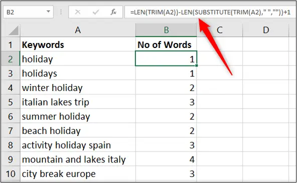
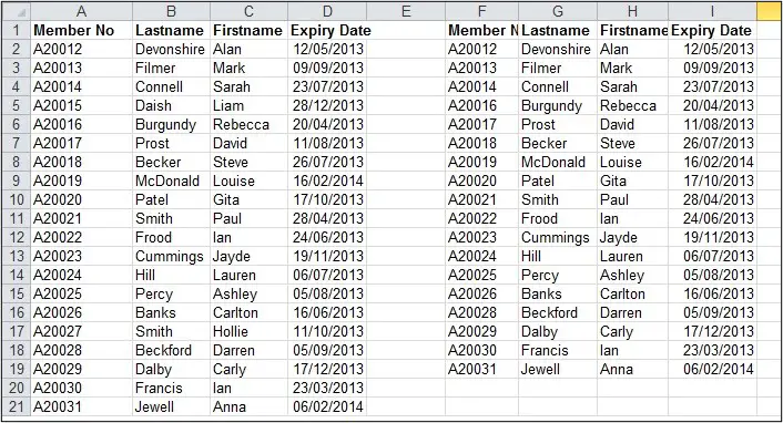
Working recently at a large Internet company they needed to find how many words were in a cell. This was because they had imported hundreds of thousands of keywords that customers had used to find their site through search engines.

To analyse this data they wanted to count how many words were in each cell containing keyword searches. Excel provides many text functions for managing and manipulating the text in the cells of your spreadsheet. The following formula did the job.

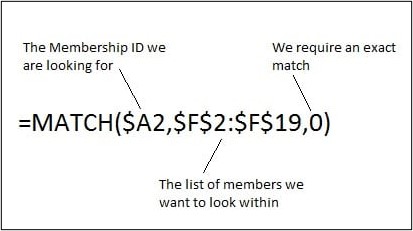
=LEN(TRIM(A2))-LEN(SUBSTITUTE(TRIM(A2),” “,””))+1

This formula subtracts a version of the cell without spaces between each word from a version still with spaces. This finds out how many spaces there are. There will be one less space than there are words so the resulting answer has a 1 added to it to find how many words there are.

The LEN function is used to find how many text characters are in the cell.
The SUBSTITUTE function is used to replace the spaces between each word with nothing making one long word.

The TRIM function is used to remove any spaces at the beginning or end of the cell content. This cleanses the cell of any erroneous spaces put in by user error, or error on import.

Count the number of words in a cell
[Read more…] about Count the Number of Words in a Cell

Excel VLOOKUP Trick – No More Counting Columns

In this post, we look at a neat Excel VLOOKUP trick to select a column for the data to return instead of specifying a column index number.

This is one of the biggest frustrations for beginners to VLOOKUP and for users who work with wide data sets. Counting the columns to enter the correct index number is not ideal.

Well, this simple trick removes that hassle and will mean you only have to click the column now. Let’s see how to do this.

Watch the Video

[Read more…] about Excel VLOOKUP Trick – No More Counting Columns

What You Need to Know About Dynamic Array Formulas in Excel

Excel dynamic array formulas things to know

Dynamic array formulas were released in 2020 to Microsoft 365 users of Excel only. They are incredible and have changed the way that many formulas are written.

Using arrays in Excel formulas is not new. They have always been possible, but apart from a few exceptions, you would need to press Ctrl + Shift+ Enter to run them. This gave them the name CSE formulas. They could also be slow and awkward to use, and certainly not dynamic.

This article will explain what you need to know about these dynamic array formulas and how to use them effectively.

Watch the Video

[Read more…] about What You Need to Know About Dynamic Array Formulas in Excel

Shrinking Drop-Down List using Dynamic Array Formulas

Shrinking drop-down list in Excel with dynamic array formulas

In this tutorial, we will create a shrinking drop-down list using the dynamic array formula engine and the FILTER function.

This is an awesome technique. Every time an item is chosen in the list, the list reduces and previously selected items are not shown.

In this example, we have a table of workers and a table of chores.

Table of workers and a table of chores

We will create a drop-down list of workers names to assign to the chores. Each time a name is assigned the list will reduce to show only the remaining names.

Watch the Shrinking Drop-Down List Video

[Read more…] about Shrinking Drop-Down List using Dynamic Array Formulas

Compare Two Lists in Excel to Highlight Matched Items

In this post, we will look at how you can compare two lists in Excel to highlight matched or unmatched items.

We will first identify the items that appear in both lists, and then look at how to highlight the items that appear in the first list but are missing from the second list.

The MATCH function will be used to compare both lists and will return if a record is found, or is missing. The MATCH function returns the relative position of an item in a list. If it cannot find the item, it will return the #N/A error message (learn more about the MATCH function).

Two lists to compare in Excel for matching items

Compare Two Lists in Excel to Highlight Matched Items

  1. Select the range of cells in the list you want to format.
  2. Click the Conditional Formatting button on the Home tab of the Ribbon and select New Rule from the list.
  3. Click the Use a formula to determine which cells to format option and enter the formula below in the box provided.

Because we are applying the Conditional Formatting to the entire row, the dollar signs are important to fix different elements of the cell references.

MATCH function to compare two lists in Excel
MATCH function used in a Conditional Formatting rule
  1. Click the Format button and select the formatting of your choice.
  2. Click Ok
Formatted rows for the matching items between two lists

Compare and Highlight the Missing Items

Instead of highlighting the duplicate items when we compare two lists, this function can be altered slightly to highlight the items that are unique to the first list.

Follow the steps as before but use the formula below for the Conditional Formatting rule.

Formula to compare two lists in Excel and identify missing items

The ISNA function is used to return true if the #N/A error message is returned. Because #N/A is returned if the Match function cannot find a record, this formula identifies the missing items in a list.

Missing items highlighted by Conditional Formatting rule

This tutorial showed how the MATCH function could be used to compare two lists and highlight matched or matching items.

Depending on the end goal, Excel offers a few methods to compare lists. Using Merge Queries in Power Query is a great alternative. The FILTER function with COUNTIFS is another.

  • « Go to Previous Page
  • Page 1
  • Interim pages omitted …
  • Page 3
  • Page 4
  • Page 5
  • Page 6
  • Page 7
  • Interim pages omitted …
  • Page 20
  • Go to Next Page »

Primary Sidebar

Recent Posts

  • TEXTSPLIT in Excel: 9 Practical Examples You Can Use Today
  • Create Custom In-Cell Bar Charts in Excel
  • Excel SWITCH Function – Nested IF Function Alternative
  • Sum Formulas Only in Excel
  • How to Calculate Age in Excel
Advanced Excel Success book

Footer

Contact

[email protected]

LinkedIn Twitter YouTube

Useful Links

  • Home
  • Excel Online Courses
  • Tutorials
  • Sitemap
  • Privacy Policy
  • Jobs by Jooble

Course Topics

  • Blog
  • Charts
  • Courses
  • Dashboards
  • Downloads
  • Excel Tips
  • Formulas
  • Mail Merge
  • Office
  • PivotTables
  • Power BI
  • Power Pivot
  • Power Query
  • VBA

Join Our Mailing List

© Copyright 2009 Computergaga · All Rights Reserved ·