If you’ve ever extracted from messy text strings, you’ve probably spent far too much time wrestling with LEFT, MID, RIGHT, and FIND formulas.
TEXTSPLIT changes all of that.
Instead of performing formula gymnastics with the likes of MID and FIND, TEXTSPLIT can instantly convert a text string into a dynamic array that Excel can work with. Due to this, TEXTSPLIT has become one of the most useful text functions in modern Excel.
In this article, we’ll explore practical examples that show how TEXTSPLIT can simplify text manipulation and unlock more powerful dynamic array solutions.
Download the practise file to follow along.
Get to Know the TEXTSPLIT Function
Let’s have a quick overview of the TEXTSPLIT function syntax, and then we will get into the practical applications for its use.
TEXTSPLIT is a simple function to get started with, but can seem daunting at first as it has many arguments.
TEXTSPLIT(text, col_delimiter, [row_delimiter], [ignore_empty], [match_mode], [pad_with])
- Text: The text that you want to split.
- Col delimiter: The characters that determine where to separate into columns. This argument is optional, but if omitted, the row delimiter must be provided.
- Row delimiter: The characters that determine where to separate into rows. An optional argument, but if omitted, the col delimiter must be provided.
- Ignore empty: Use FALSE to return blank values for any consecutive delimiters or TRUE to not return blank values. By default, blanks are returned in place of empty values.
- Match mode: Enter 0 for a case sensitive match on the delimiter or 1 for case insensitive. By default, a case sensitive match is performed.
- Pad with: When data is missing, #N/A errors are returned in place of cells with missing data. With this argument, an alternative value can be used to pad instead of the #N/A error.
1. Simple TEXTSPLIT Example
Beginning with a simple example of TEXTSPLIT, we have some text data separated by hyphens. Our goal is to split the text at each instance of a hyphen.
This data is consistent and there are two hyphens in each value, so our result should split the text into three columns.
=TEXTSPLIT(B3, "-")
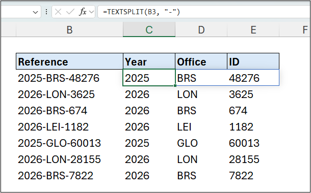
The TEXTSPLIT formula was entered in cell C3 and then filled to the other rows. This example would not work correctly if you referenced range B3:B9 in the formula.
Later in this article, we will cover how to do this with a single formula and avoid the array of arrays issue, but for now we write a separate formula for each row.
2. Use INDEX to Extract Specific Text from the String
One obstacle that inhibits me from using the TEXTSPLIT function as much as I would love to, is that we cannot spill formulas within Excel tables – and I love to use Excel tables.
However, although TEXTSPLIT returns an array of values, we do not need to spill all values to the grid, and we will see a few practical examples of TEXTSPLIT being used in this manner throughout this article.
For this example, let’s use the fabulous INDEX function to extract specific text from the array returned by TEXTSPLIT.
=INDEX(TEXTSPLIT([@Reference],"-"), , 2)
The formula extracts the office code only from the reference. It also uses a table reference “[@Reference]”, which is ok as TEXTSPLIT is not spilling multiple values.
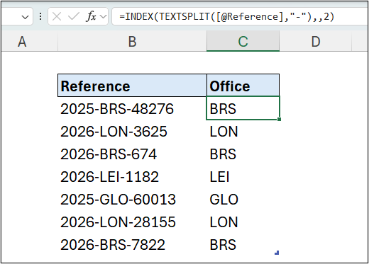
For the result in range C3, the array {“2025”, “BRS”, “48276”} was returned by TEXTSPLIT, and INDEX returned the text in the second column of that array. In the INDEX formula, you can see the consecutive commas where the row index argument was ignored.
You may be thinking that a MID formula like the following would be easier in this example. And you would be correct, as the values are quite consistent.
=MID([@Reference],6,3)
However, if we are working with an irregular string and the starting position of a character and/or the number of characters to extract is unknown, things get more tricky.
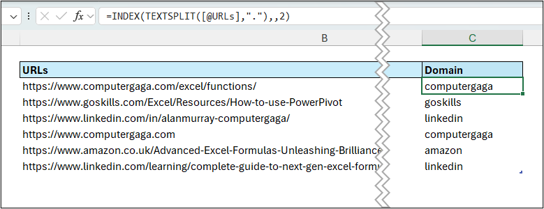
In the following formula, the domain is extracted from each URL. The domains are irregular in length but that is not a concern for TEXTSPLIT and INDEX.
=INDEX(TEXTSPLIT([@URLs], "."), , 2)
Without the use of TEXTSPLIT, we would be looking at using a TEXTAFTER and TEXTBEFORE combination like the following.
=TEXTBEFORE(TEXTAFTER([@URLs], "."), ".")
Or this beautifully complicated MID and FIND combination.
=MID(
[@URLs],
FIND(".", [@URLs])+1,
FIND(".", [@URLs], FIND(".", [@URLs])+1)-FIND(".", [@URLs])-1
)
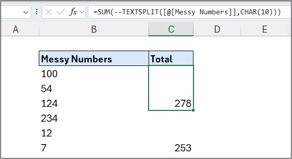
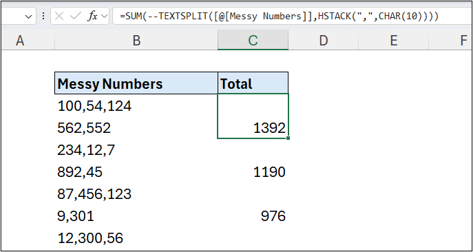
3. SUM Messy Numbers
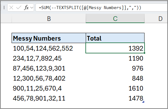
You’ve received a data export that contains lists of numbers stored in single cell. How are you going to easily sum these numbers?
Let’s use a TEXTSPLIT formula to split the numbers at the comma delimiter, the double negative to convert them to positive values (TEXTSPLIT results are always a text data type), and then SUM to do what it does best.
=SUM(--TEXTSPLIT([@[Messy Numbers]], ","))
4. TEXTSPLIT with Multiple Delimiters
By using an array of constants, the Excel TEXTSPLIT function can handle multiple delimiters.
In this example dataset, we have affiliate URL’s and we are looking to extract three items of information from each of them.
- Course name such as ‘advanced excel tricks’ or ‘ultimate excel course’
- Coupon code such as ‘FORMULAPRO10’ or ‘TRICKS30’
- and the source such as ‘linkedin’ or ‘blog’
There are multiple delimiters used in each URL. For example, the course names can be found between a / and a ?. Then the coupon code can be found between an = and an &. And the source trails behind the final =.
The following formula produces an array containing the results we need, and will extract from.
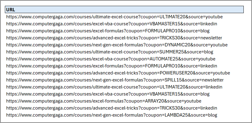
=TEXTSPLIT(B3, {"/", "?", "=", "&"}, , TRUE)
This TEXTSPLIT formula is splitting at four different delimiters, entered as an array of constants (signified by the curly braces). Consecutive delimiters create empty values in TEXTSPLIT, so TRUE is used for the ignore empty argument to ensure that an empty cell is not returned for the consecutive // in each URL.
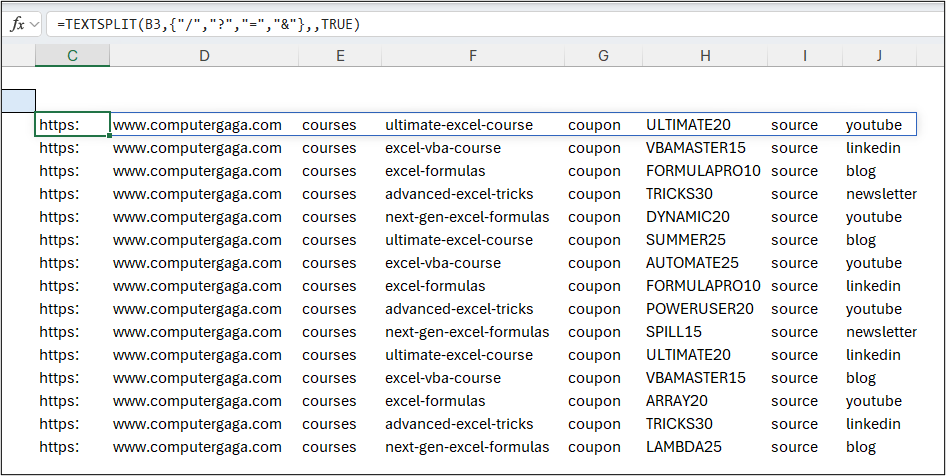
With this result, you can probably how we can grab the text that we need from the returned array. INDEX can be used, as we did previously.
For example, using an INDEX of column 4 would extract the fourth element, which is the course name.
=INDEX(TEXTSPLIT(B3, {"/", "?", "=", "&"}, , TRUE), , 4)
Index 6 is the coupon code.
=INDEX(TEXTSPLIT(B3, {"/", "?", "=", "&"}, , TRUE), , 6)
And we could repeat this method for the source, but to mix things up, let’s use the TAKE function to return the final column from the array – the source name.
=TAKE(TEXTSPLIT(B3, {"/", "?", "=", "&"}, , TRUE), , -1)
Of course, you could tidy the results further, such as removing the hyphens from the course name using the SUBSTITUTE function, or changing the case of the results using UPPER or PROPER, but that is not the focus of this article, so let’s move on to another example.
5. Handling Unprintable Characters in TEXTSPLIT
To use unprintable characters, such as the line break character for a delimiter with TEXTSPLIT, the CHAR function is utilised. The line break, or line feed, character is char 10.
To sum the messy numbers from earlier, but this time separated by a line break, the following formula is used.
=SUM(--TEXTSPLIT([@[Messy Numbers]], CHAR(10)))
6. Stacking Characters with HSTACK
It could be that you have multiple delimiters for TEXTSPLIT to use, which include unprintable characters. Now, we cannot use a function such as CHAR within an array of constants, so how can we use an array of constants and CHAR in one TEXTSPLIT formula?
We can stack them with HSTACK.
The following formula handles these messy strings easily. HSTACK is used to create an array from the comma and the CHAR(10), which is given to TEXTSPLIT to work with.
=SUM(--TEXTSPLIT([@[Messy Numbers]], HSTACK(",", CHAR(10))))
7. Array of Arrays Issue
We have seen plenty of examples of TEXTSPLIT splitting text across multiple cells, so producing a multi-column array of values, that is then used by a function like INDEX or spilt to the grid.
When returning multiple values like this, TEXTSPLIT function cannot also spill the formula results down as it cause something known as the ‘array of arrays’ issue.
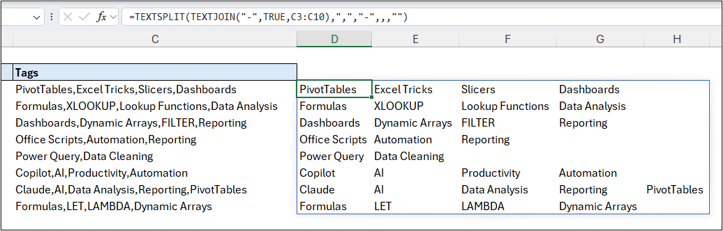
Take the following data, and our goal is to find the most commonly used tags on our website. We want to achieve this all in one formula – because that is true next-generation Excel formula work.
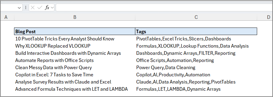
First, we need to split the tags by their comma delimiter.
We want to do this with one formula for all rows – no dragging the formula to duplicate it for each row.
The following formula is not working. It is only returning the first tag in each list. This is the array of arrays issue at work. It cannot return the entire array for each row.
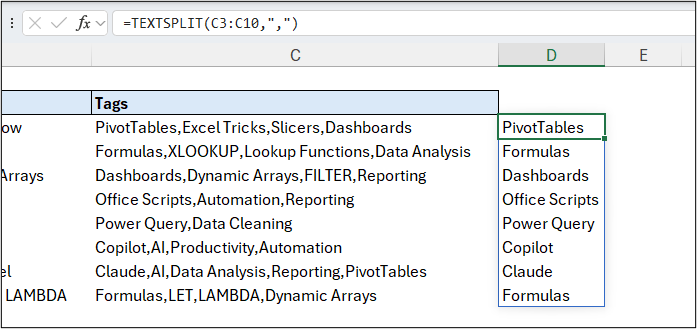
Hopefully, this issue will be solved in the future, but for now, the easy fix is to combine the tags into a single array first before splitting it.
The following formula uses the TEXTJOIN function to join all rows into a single array separated by a hyphen. The hyphen is then added to our TEXTSPLIT formula as our row delimiter.
=TEXTSPLIT(
TEXTJOIN("-", TRUE, C3:C10),
",", "-")
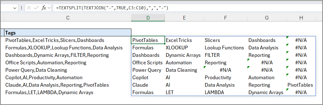
The result is all tags produced by a single formula. Each blog post tags are in separate columns and each blog post in separate rows.
However, we do have error messages amongst the resulting array, so let’s clean that up next.
8. Padding missing values
The TEXTSPLIT Excel function has an argument to handle these error values – the pad with argument.
In this formula, an empty string is used for the pad with argument. This is the final argument, so two consecutive commas were used to move past two redundant arguments.
=TEXTSPLIT(
TEXTJOIN("-", TRUE, C3:C10),
",", "-", , , "")
We now have a result for the entire range from a single formula.
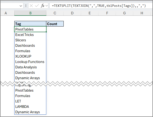
9. Single Cell Formula with GROUPBY
To complete our task of reporting on the most commonly used tags, we will use the separated tags within a GROUPBY function and count their occurrences.
First, we will refine how all the tags are returned to separate cells. In the following formula, we have simplified the previous version of the formula.
Now, the comma is used as the delimiter by TEXTJOIN when combining all rows. This is the same delimiter as we have between each tag already, and this is fine, as we do not need the distinction of which blog post it belongs to. We simply want a list of all tags used.
For the TEXTSPLIT function, the comma is now used for the row delimiter, so the blog post tags are in separate cells down a column.
=TEXTSPLIT(TEXTJOIN(",", TRUE, tblPosts[Tags]), , ",")
This formula can now be used within GROUPBY.
We need to use these results both for the row label and for the value to count within GROUPBY, so we can use the LET function to avoid repeating the TEXTSPLIT and TEXTJOIN calculation twice in the formula.
=LET(
tags, TEXTSPLIT(TEXTJOIN(",", TRUE, tblPosts[Tags]), , ","),
GROUPBY(tags, tags, COUNTA)
)
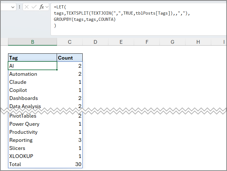
The TEXTSPLIT and TEXTJOIN calculation results are assigned to the name tags. This is then used in the GROUPBY function and COUNTA is used to count the number of occurrences of each tag.


Leave a Reply