Highlight Rows when Value Changes – Excel Conditional Formatting

In this blog post, we create a Conditional Formatting rule to automatically highlight rows in an Excel list at each value change.

I’ve got multiple guests from the same company attending an event and I want each company section to stand out. The default banded rows of Excel Tables does not help with reading my attendee tracker.

For this example, I want to highlight groups of rows – each company in my list.

Let’s create a Conditional Formatting rule to automatically highlight each company section. The rule will format the entire row based on the company name changing from the previous row.

This is much easier to read compared to the classic banded row formatting used by Excel tables.

So, how can we do this?

1. Identify the Value Change

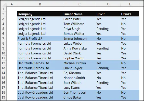
Our first task is to identify the change in company name.

We can achieve this with a simple formula that checks if the current cell value is not equal to the previous rows cell value.

=$B3<>$B2

In this example, our first data row is in row 3 of the sheet, so we are comparing the first cell value in that column (B3) against the previous rows value.

In column G, the formula returns TRUE whenever there is a value change.

Excellent!

But that is just the first company name in a section, and the company name may be stated 2, 3, 4 times before that value changes.

So, we need to progress the formula and identify the group, not just the first one.

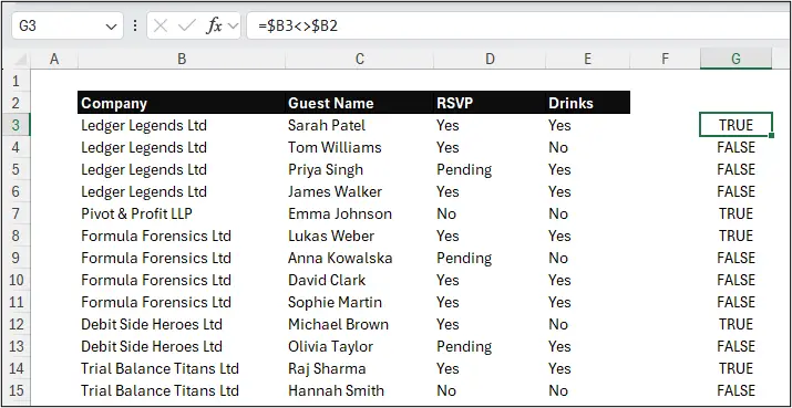
2. Flag Each Section Where Formatting Changes

We will convert the TRUE and FALSE values to 1 and 0 using the N function in column G. This function will convert TRUE values to 1 and anything else to 0, giving us the numeric values we need for the next step.

Then, we’ll use a cumulative sum formula to sum the values one row at a time. This will cause the numbers to increment at each group change. The following formula was used in cell H3, and copied down.

=SUM($G$3:$G3)

Now we are getting somewhere.

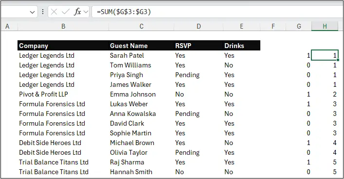
All values except 0 are evaluated to TRUE by Excel, so for our Conditional Formatting rule, we will need to change these incremental numbers into 1 and 0 at each value change.

3. Return 1 and 0 for Alternating Sections

For this, we can use the MOD function. This function returns the remainder, after one number is divided by another. If we divide each number by 2, the odd numbers will return a remainder of 1 and the even numbers will return a remainder of 0 – giving us our 1’s and 0’s.

=MOD(SUM($G$3:$G3), 2)

4. Final Conditional Formatting Formula

We’ve successfully identified the different companies at each value change. And this formula will automatically update as rows are inserted, deleted, or added.

However, the formula is not ready for Conditional Formatting just yet.

To highlight rows based on a formula, we’ll need to bring our formulas used in two different columns together, and expand the original single cell test of $B3<>$B2 to work for the entire range of the table.

The final formula, adapted for the Conditional Formatting rule, is the following.

=MOD(SUM(--($B$3:$B3<>$B$2:$B2)), 2)=1

Here, we have our two cumulative ranges that test if the previous rows value is different to the current rows value. The result of the MOD is then compared to 1. This identifies formulas that return odd numbers.

This second formula can then be used for a Conditional Formatting rule to highlight rows where there is an even number.

=MOD(SUM(--($B$3:$B3<>$B$2:$B2)),2)=0

5. Apply Conditional Formatting rules

To apply Conditional Formatting to the rows of the table:

1. Select all rows of the table, except the header row.
2. Click Home > Conditional Formatting > New Rule.
3. Choose Use a formula to determine which cells to format.
4. Paste the first formula into the box provided, and then click Format to choose your formatting.
5. With the first rule created, click Duplicate Rule, change the 1 on the end to a 0, then choose a different colour from the Fill tab of the Format Cells dialog.

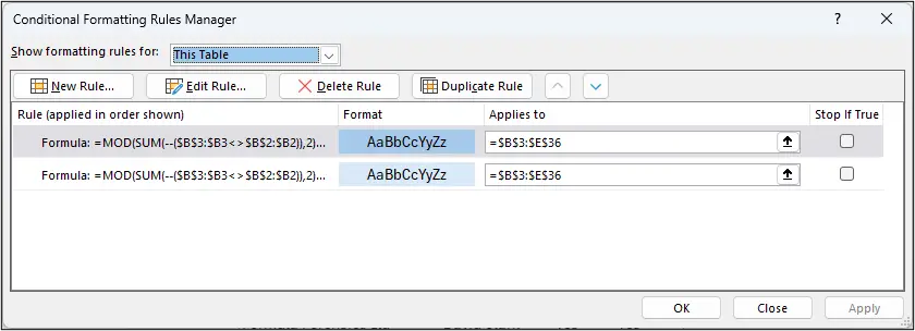
We now have formatting that will automatically highlight rows each time the value changes in column B.

Simple Conditional Formatting trick. Huge difference.