The VLOOKUP function will look down the leftmost column of a table and return a value from a specified column index number. To create a two way lookup formula, we will need something more flexible.

The INDEX and MATCH functions can be used to create a two way lookup that looks down a column and across a row.

These two functions used together create a very versatile and dynamic lookup formula. A far cry from the rigid structure of VLOOKUP.

If you are using Excel 365 or Excel 2021 version of Excel, you can also create a two way lookup with the XLOOKUP function. This is awesome and you should definitely check it out. But for now we will stick with the INDEX MATCH combination, and INDEX is the greatest function of all.

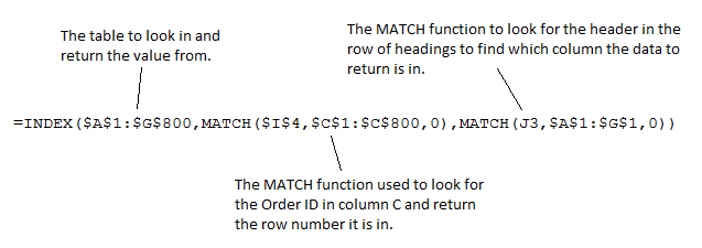
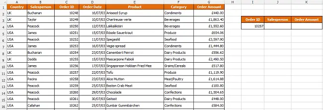
In the example, below we wish to look for an order using the ID, and return the salesperson’s name and the order amount using the same lookup formula in both cells.

The INDEX and MATCH Functions

The two way lookup formula is a combination of the INDEX and MATCH functions. These two functions are fantastic and have many uses in Excel. Let’s have a little look at the two of them first.

The INDEX function is used to return a value from a specified column and row. In addition to its use in a two way lookup, this function is used when working with form controls on a spreadsheet.

When used to return a value it is written as below.

=INDEX(array, row_num, [column_num])

This function wants to know the row and column number of the cell containing the value to return.

The MATCH function is the driving force in this formula. It will be used to find and return the row and column numbers for the INDEX function. INDEX can then return the value from that cell.

The MATCH function is heavily used in many lookup and reference situations to add extra muscle to the likes of VLOOKUP, or Conditional Formatting.

It’s structure is as below.

=MATCH(lookup_value, lookup_array, [match_type])

The lookup value is the value to search for.

The lookup array is the range of cells to search in.

Match type is the type of lookup to use. You can select an exact match, or one that finds the closest match if it cannot find the value you are looking for.

Create the Two Way Lookup Formula in Excel

In this example, the formula below is entered into cell J4 and copied into K4.

Watch the Video

In this Ultimate VLOOKUP guide we begin with an introduction to the VLOOKUP function for newbies, and then look at some more advanced examples of its use.

The VLOOKUP function is one of the most commonly used and powerful functions in Excel. It is often misunderstood and can be tricky to use especially if you are not confident with Excel formulas.

There are many reasons people use VLOOKUP. These range from dynamically linking worksheets, to comparing lists for missing items, to improving and speeding up data entry.

Our guide shows you how to combine VLOOKUP with other Excel functions to achieve more powerful searching within a spreadsheet.

• Introduction to the VLOOKUP Function
  This introductory VLOOKUP guide shows you when and how to use this function. Understand its anatomy and how to write VLOOKUP formulas to accomplish common spreadsheet tasks.
  
• Looking for a Value to the Left (Video)
  A limitation to the VLOOKUP function is that it can only look down the first column of a table and return data to its right. This tutorial looks at using the INDEX and MATCH functions to return data from a column to the left.
  
• Create a Two Way Lookup
  Used by itself, VLOOKUP will look at the first column of data in a table and bring back a value from another column on the same row. This is a very rigid lookup.
  
  This VLOOKUP tutorial looks at how to create a two way lookup to look for a value in a column, but also automatically find the column containing the value to return.
  
• VLOOKUP with a Conditional Lookup Table
  If your workbook contains multiple lookup tables, you may want a user to specify which table VLOOKUP should use as the table array.
  
  This tutorial looks at how you can create a VLOOKUP that uses a table that the user picks from a list.
  
• Create a Multiple Condition Lookup Formula
  The VLOOKUP function is typically used to search for a record using a unique ID such as a part code, or customer ID. However you may need to match multiple columns to ensure you have found the correct record.
  
  This special VLOOKUP tutorial will look at how to create a lookup that matches the data in multiple columns.
  
• Create a Case Sensitive Lookup Formula
  The lookup value in the VLOOKUP function is not case sensitive. Learn how to create a case sensitive lookup formula that will find an exact match for the lookup value in the list.
  
• Create a Picture Lookup
  If you have a list containing images such as a product list with a picture in one of the columns, you may want to create a lookup that returns the picture.
  
• Find the Cell Address of a Value
  Looking up a value and returning data relating to it is great. But you may want to return the cell address of the value you are looking for.
  
• Compare Two Lists Using VLOOKUP
  A common Excel task is to compare two lists to find matching or missing records. This tutorial demonstrates using VLOOKUP with the IF function and Conditional Formatting to compare lists.

If you have found this ultimate VLOOKUP guide useful, why not check out more Excel formulas.

The FILTER function in Excel is a dynamic array function available to Excel 365 users and Excel Online only.

This is an extremely versatile and powerful function – and is possibly the best function in Excel.

It is the formula equivalent of the extremely useful filter feature of Excel. It will return a range dependent upon criteria that you specify.

This range can be returned to a worksheet but also embedded inside other formulas.

The potential for this is huge. With the FILTER function providing the ranges for other formulas, and also our charts and data validation rules etc. This function has changed the game forever.

In this guide, we will introduce you to the FILTER function with different examples. The potential for this function is so vast, that you need to explore it yourself also.

Download the file used in this tutorial to follow along.

Watch the Video

How to Use the FILTER Function in Excel

Let’s take a look at the classic use of the FILTER function. To automatically output a range of data that meet specified conditions.

For example, we have a list of training (columns A:C) with a date column for when that training requires renewing. It has been formatted as a table named training.

And we want to return a list into the range to the right (columns F and G) of the names and expiry dates of the training that is overdue.

So in cell F5, we will use the FILTER function.

The FILTER function accepts three arguments – array, include and if_empty.

Array: The range of values you want to be filtered.

Include: The filter criteria. Boolean expressions which will determine what rows or columns to return.

If Empty: The action to take if no results are returned by the filter. This is an optional argument.

The following formula can be used to return the name and expiry date.

=FILTER(training[[Name]:[Expiry Date]],training[Expiry Date]<TODAY(),"All up to date")

The Array is the name and expiry date columns of the table (table references are used in the formula) because this is the information we want to be returned.

The following criteria is used for the Include argument.

training[Expiry Date]<TODAY()

This ensures that the expiry date is before today’s date.

Finally the text “All up to date” will be returned if the FILTER function returns no records.

The following results are returned. A blue border is shown around the “spill” array.

Because dynamic arrays have been used here, all results are returned by one formula. However, to edit the formula, you must do this in the first cell of the array only (cell F5).

Excel FILTER Function with Multiple Criteria

The previous FILTER function example has only one criterion – if the expiry date was in the past.

However, let’s test the training course as well. In cell G2 there is a drop-down list for the different courses – call handling, Excel and first aid.

We want the FILTER function to return the name and expiry date of the training that has expired AND for the course listed in cell G2.

To do this we need to surround both logical tests in brackets and multiply them.

This is the complete formula.

=FILTER(training[[Name]:[Expiry Date]],(training[Expiry Date]<TODAY())*(training[Training]=G2),"All up to date")

And here is the Include argument isolated so that it is easier to understand.

(training[Expiry Date]<TODAY())*(training[Training]=G2)

The formula returns the following results when Excel is selected.

Changing the course in the drop-down would immediately produce the results for that course. Here are the results for First Aid training.

Why multiply them?

Whenever you want to perform And logic and only include the results where all logical tests are equal to true, you must multiply each boolean expression.

The reason for this is because each test is conducted separately.

So all the expiry dates that are previous to today’s date return a true. This is a snapshot of how the first 11 rows of our data are evaluated.

{TRUE;FALSE;FALSE;FALSE;TRUE;TRUE;TRUE;TRUE;TRUE;FALSE;FALSE}

And then all training that is equal to the value in cell G2 return a true.

{FALSE;FALSE;TRUE;TRUE;FALSE;TRUE;FALSE;TRUE;FALSE;FALSE;TRUE}

The two arrays are then multiplied. The rows that are equal to 1 are the results that are returned.

{0;0;0;0;0;1;0;1;0;0;0}

So multiplying the expressions ensures that all tests must equal to True to evaluate to 1.

How about OR logic?

If you wanted a scenario where only one of the logical tests must equal true to be included, then wrap each boolean expression in brackets and add them with the plus operator (+) instead.

Tidy this up with the IF Function

The previous example works great, but only if cell G2 is populated with one of the course names.

If it is not, then the text “All up to date” is returned. And this is not true.

The following formula uses an IF function to test if cell G2 is empty. If it is, then use the FILTER function with no test on a course name, but if it isn’t then use the FILTER function that does test the course name in cell G2.

=IF(G2="",FILTER(training[[Name]:[Expiry Date]],training[Expiry Date]<TODAY(),"All up to date"),FILTER(training[[Name]:[Expiry Date]],(training[Expiry Date]<TODAY())*(training[Training]=G2),"All up to date"))

This formula may seem daunting due to its size. But really it is just two FILTER function being controlled by the IF function and the test on cell G2.

Breaking the formula up onto different lines can make it easier to understand.

=IF(G2="", FILTER(training[[Name]:[Expiry Date]],training[Expiry Date]<TODAY(),"All up to date"), FILTER(training[[Name]:[Expiry Date]],(training[Expiry Date]<TODAY())*(training[Training]=G2),"All up to date"))

Use the FILTER Function with Other Excel Functions

The previous example showed the FILTER function with the IF function.

One of the great advantages of the FILTER function is that it returns an array based on criteria – like a super lookup. And this array could be used in any Excel function.

In the range below we will count the number of training that has expired for each course.

To do this we will combine FILTER with the COUNTA function.

FILTER could be combined with any function – SUM, LARGE, VLOOKUP, MEDIAN making it extremely flexible.

The formula below returns the count of expired training for each course.

=COUNTA(FILTER(training[Name],(training[Expiry Date]<TODAY())*(training[Training]=I1)))

The formula returns the names if the date has expired and training is equal to the value of I1. These names are then counted by COUNTA.

The Excel FILTER function is incredibly useful and will change the way people use formulas.

There are so many scenarios where this function will come in handy. For example, below is a video on using it to create a searchable drop-down list.

Some of these special scenarios will become clear as you play around with it and use it in your workplace.