In this blog post, we look at 5 examples of the INDIRECT function in Excel. This is a very misunderstood function. It is an incredibly useful function.
Prefer to watch the video? The video tutorial below will demonstrate all 5 Excel INDIRECT function examples.
Download the sample INDIRECT function workbook to practise the examples.
What is the Excel INDIRECT Function?
Before I delve into these different INDIRECT examples, let’s learn the anatomy of this wonderful function and how it operates.
The INDIRECT function is one of the lookup functions of Excel. And it’s purpose is to return a reference which is specified by text (typically some text in the cell of a worksheet).
This becomes really useful to create references to other sheets, named ranges and tables from a cell value. You will see these in the following examples.
The Excel INDIRECT function looks like below.
=INDIRECT(ref_text, [A1])
- Ref_text: A reference to a cell that contains, or partially contains, an address.
- A1: This argument is optional. It determines the type of reference for INDIRECT to use. If you type TRUE then the normal A1 style is used. If you type FALSE, the R1C1 style is used.
Ok, let’s get stuck into these tutorials.
1. Using INDIRECT with Named Ranges
A great use for INDIRECT is with names. There are two main types of names in Excel – tables and named ranges.
The concept of using names for simpler referencing has huge benefits, and when you understand INDIRECT those benefits are amplified. This example demonstrates the Excel INDIRECT function with named ranges.
In the example below, cell G4 contains the total for the sales of the region mentioned in F4. In this image, it is for Cardiff.
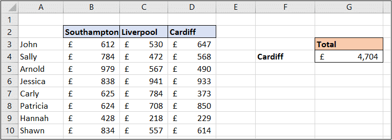
This total was achieved using the formula below.
=SUM(INDIRECT(F4))
Each range of values has been named after the region. For example range D3:D10 is named Cardiff, and range B3:B10 is named Southampton.
The Excel INDIRECT function returns the value from F4. This value is then converted from text to a reference so that the SUM function can add the values from the named range.
Without INDIRECT the SUM function would not use the value in F4 as a reference to the named range.
Watch this video for an example of the INDIRECT function in Excel with table references.
2. INDIRECT to Dynamically Reference other Worksheets
In this example, we want to reference a different worksheet within a formula, which is another SUM function. The worksheet we are summing values from is dependent upon the value in a cell. So once again, INDIRECT is needed.
The image below shows the summary sheet, and cell B3 contains the name of the sheet that we will be summing from. The beauty of this technique is that if someone changes the value in cell B3, it then sums from that sheet.
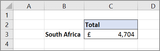
The formula below has been used in this example. In each sheet the values to be summed are in range C4:C11.
=SUM(INDIRECT("'"&B3&"'!C4:C11"))
The apostrophes have been used in the formula to enclose the sheet name. If a sheet name contains spaces, such as South Africa, apostrophes are required.
3. Return the Last Value from a Row
In this example, we will look at using an R1C1 style reference with INDIRECT to return the last value from a row.
In the image below, the formula in cell F3 is returning the last value in row 10. This ensures that as new months (columns) are added to the range, it always retrieves the current months value.
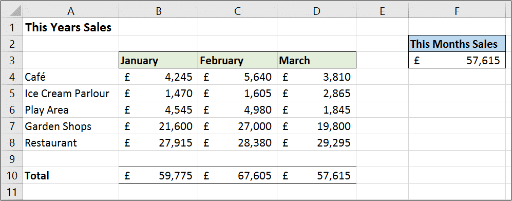
The formula below has been used in cell F3. By using an R1C1 reference style instead of the traditional A1 style, we can refer to the column numerically. The COUNTA function has been used here to count the non blank cells of row 10, therefore returning the last column.
=INDIRECT("R10C"&COUNTA(10:10),FALSE)
This is concatenated onto the R10C part to complete the reference as row 10 and column 4.
The FALSE part of the INDIRECT formula requests the R1C1 style reference.
4. Excel INDIRECT Function with VLOOKUP
It feels necessary to include an example of using INDIRECT with the VLOOKUP function. For this example, INDIRECT will be used to create a conditional lookup table.
Of course, techniques such as this will work with lookup formulas such as XLOOKUP and FILTER also.
In the image below, a VLOOKUP function has been entered into cell B3 to return the sales value for Jessica (B1) and Cardiff (B2).
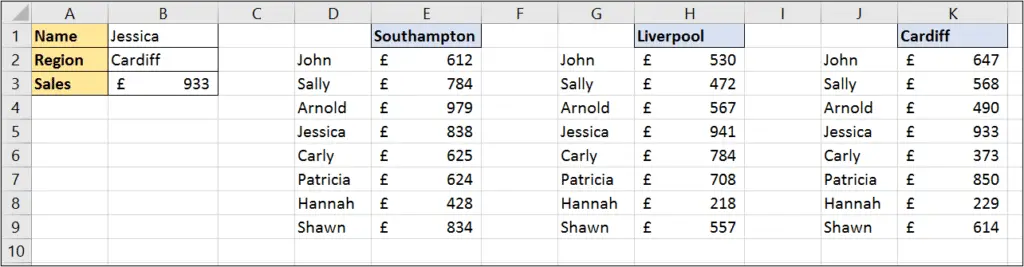
Each lookup table has been named appropriately as Southampton, Liverpool and Cardiff. Just like in the first example of this blog post, INDIRECT has been used to convert the value of cell B2, to a reference to a named range.
The formula below, uses VLOOKUP to return a value from a table, specified by the value in cell B2. The INDIRECT function is entered into the table array argument of VLOOKUP.
=VLOOKUP(B1,INDIRECT(B2),2,FALSE)
5. Create Dependent Drop Down Lists
Another brilliant use of INDIRECT is to create dependent drop down lists. This is a great technique if you work with large lists.
You can break the large list up into multiple smaller lists and then make them dependent on one another. So the selection from one list determines the options that appear in the next list.
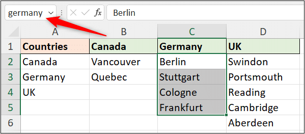
In the image below, each range of cities has a name defined that matches the country name. It is essential for this technique, that the country name in range A2:A4 matches the named range for each country. This is because INDIRECT will reference the named range from the list item.
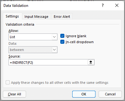
The following Excel INDIRECT formula can then be used for the list source in the Data Validation window. Cell F2 contains the value from the first drop down list.
=INDIRECT(F2)
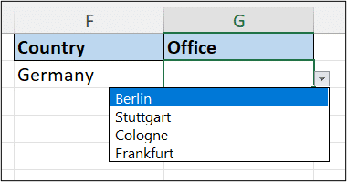
Now, when an option is chosen from the first list, the second list shows only the options that relate to that selection.
Check out this video on how to create multiple dependent drop down lists.
If any of these INDIRECT examples are not clear, check out the video at the top of this blog post which will show you exactly how each formula is done.


Liked your approach of providing the file, but not filling in the solutions, to inspire practicing !
Your tutorials are really nice to follow and obviously based on good teacher practices, congrats !
Thank you very much Danny. Much appreciated ?
INDIRECT is a terrible function to use, it is volatile, and the argument is often static text, and so does not update if the referred to cell(s)/sheet(s) are moved/renamed. Even if you use a named range, if it is renamed, the formula breaks.
It is definitely not a function that should be taught to novice, or intermediate users, especially when there are better options. For example, in your named ranges table example, you could use
=SUM(INDEX($A$2:$D$10,0,MATCH(F4,$A$2:D$D$2,0)))
Or with the whole table as a named range, let us say Sales
=SUM(INDEX(Sales,0,MATCH(F4,INDEX(Sales,1,0),0)))
Or better still, with the data in a table
=SUM(INDEX(tblSales[#Data],0,MATCH(F4,tblSales[#Headers],0)))
As with anything, it depends when and why you are using it. INDIRECT is definitely not terrible, it offers advantages over others. The volatility and static text are often not a problem depending on the context in which they are used.
Feel free to check out my tutorials on SUM and INDEX because conveniently you are mentioning my two favourite functions there. But because I prefer them, and they are more useful does not make INDIRECT terrible or not useful.