Nested IF formulas are extremely useful for complex decision making on a spreadsheet, but they can also be long, messy and convoluted.
This blog post explores 4 alternatives which are easier, faster and cleaner than the classic nested IF.
Watch the Video – Nested If Formula alternatives
1. The IFS Function (Nested IF in One Function)
Lets start with a function that is new from Excel 2016 called the IFS function.
This function was introduced to condense and simplify the task of writing nested IF formulas. You can avoid all of those brackets that come with opening and closing multiple IF functions.
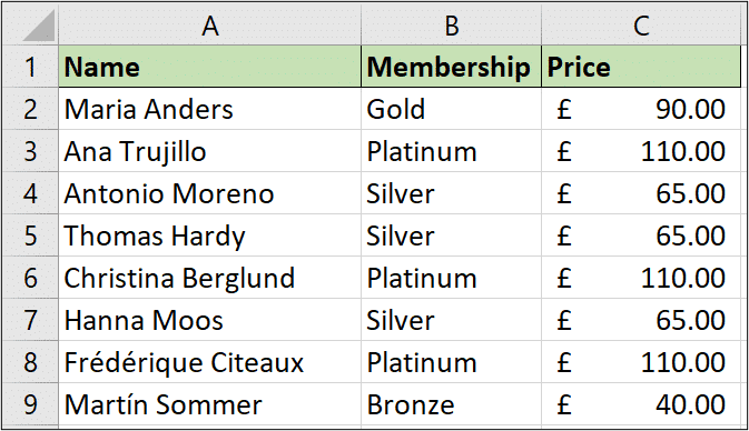
In the example below we used an IFS function to calculate the price for each membership type. There are four types of membership (platinum, gold, silver and bronze).
The IFS function tests cell B2 for each membership type and applies the correct price.
=IFS(B2="Platinum",110,B2="Gold",90,B2="Silver",65,B2="Bronze",40)
The IF and IFS functions can be used to check if a string contains text, instead of an exact match, by using the SEARCH and ISNUMBER functions.
2. Using VLOOKUP for an Exact Match
I believe an even better alternative to the IFS function for this scenario would be a lookup.
Now you can use any lookup formula that you like to achieve this. In this example I will use VLOOKUP.
By creating a lookup table (F4:G7 below) we are able to use the following VLOOKUP function to search for each membership and return the correct price.
=VLOOKUP(B2,$F$4:$G$7,2,FALSE)
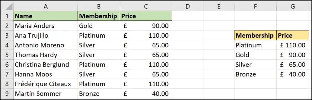
This is very compact and easier to adapt in the future. If a membership price changes, you can just change the lookup table. There is no need for someone to have to edit the formula, which you or your colleagues may not be comfortable doing 10 months from now.
3. Using VLOOKUP for a Range Lookup
In this nested if formulas alternative, we use VLOOKUP again, but this time for a range lookup.
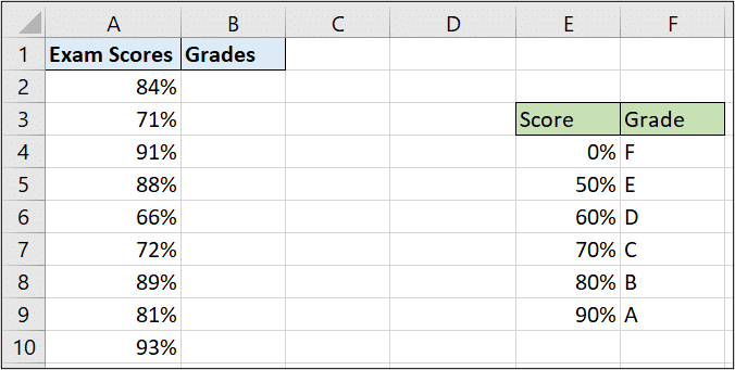
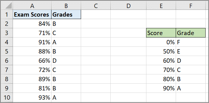
Take the example below where we have a list of exam scores and we need to assign a grade for each score.
A nested IF formulas approach could look like this.
=IF(A2>=90%,"A",IF(A2>=80%,"B",IF(A2>=70%,"C",IF(A2>=60%,"D",IF(A2>=50%,"E","F")))))
Or even like this.
=IF(AND(A2>=90%,A2<=100%),"A",IF(AND(A2>=80%,A2<90%),"B",IF(AND(A2>=70%,A2<80%),"C",IF(AND(A2>=60%,A2<70%),"D",IF(AND(A2>=50%,A2<60%),"E","F")))))
Now these formulas work perfectly. However they are complex and messy. And unless your trying to impress someone with big complex looking functions, there are better ways.
With the lookup table set up in range E4:F9 we could use this VLOOKUP function.
=VLOOKUP(A2,$E$4:$F$9,2,TRUE)
Much simpler.
This is a range lookup, so it is essential that the first column of the lookup table (column E) is in ascending order.
4. The Fantastic CHOOSE Function
This last alternative to the nested IF formula is a bit of a secret function. Many Excel users will never have even heard of the CHOOSE function.
This function will perform an action based on a specific index number. And that makes it perfect for use with form controls.
So in this example I have an interactive chart being driven from a combo box control.
The image below may look a little messy. Typically some of this data would be hidden or stored on separate sheets. It is all on one sheet here to get a better idea of how it works.
The first 7 rows have data of the top goal scorers from 4 different football leagues in the 2016-17 season. A combo box is on the left and is linked to cell A9. A selection from the 4 leagues in the combo box will produce index number 1, 2, 3 or 4 in cell A9.
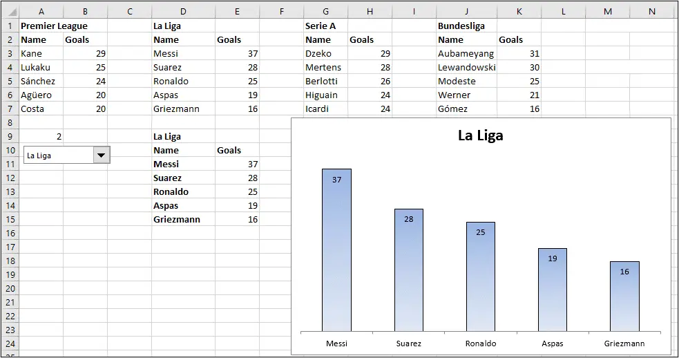
Formulas are in cells D9 and range D11:E15 returning the correct data for the chart from the combo box selection. This is easier explained in the video.
Now in the cells mentioned above we could use a nested IF like below. This is the nested IF from cell D11 which returns the name of that leagues top goal scorer.
=IF(A9=1,A3,IF(A9=2,D3,IF(A9=3,G3,IF(A9=4,J3))))
Or we could use this awesome and simple little CHOOSE function. It checks the index value in cell A9 and then returns the relevant information from its list.
=CHOOSE($A$9,A3,D3,G3,J3)
I hope you found these nested IF formula alternatives useful. Check out these other Excel formula tutorials.


october sancho 10
october sancho 20
october sancho 30
october sancho 40
october neymar 50
how could i calculate the top 3 scores for sancho in october? i have a data set where 1000 players in october and i need to sum the top three for each player for that month. i tried to do this =IF(AND(E17=C17:C21,F16=B17:B21),SUM(LARGE(D17:D21,{1,2,3}))””) but due to the last part of the if function since it says neymar at the bottom it leaves it blank.
Hi Alex, you can use SUMPRODUCT. I have videos on that function. It is marvellous.
The following formula does what you ask. It assumes the data you provide starts in A2. And that the month October is in cell F3 and the name Sancho is in E3
=SUMPRODUCT(($B$2:$B$9=E3)*($A$2:$A$9=F3)*($C$2:$C$9=LARGE($C$2:$C$9,{1,2,3}))*($C$2:$C$9))
Now there are alternative methods to this, especially because you want all months and names. But this works.
In Excel 365, if you have that, the FILTER function can be used.