This tutorial explains an Excel formula to find the least frequent value in a list. This formula will work whether the value is a number, or text. In this example we want to return the name that occurs the least.
The spreadsheet below shows a list of names with the answer in cell D2. Ross is the name that occurs the least in that list.
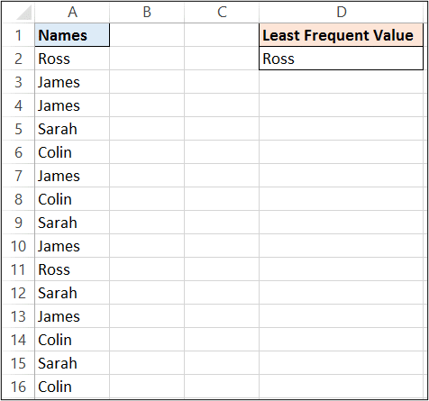
This formula returns the least frequent value from the list in A2:A16. The formula is explained below so keep reading.
{=INDEX(A2:A16,MATCH(MIN(COUNTIF(A2:A16,A2:A16)),COUNTIF(A2:A16,A2:A16),0))}
Excel Formula Explained
This formula is an array formula so you need to press Ctrl + Shift + Enter, and not Enter. This will put the curly braces around the formula. You do not type these.
Within this formula the COUNTIF functions are used to return how many times each name occurs in the list. The COUNTIF functions return the result below;
{2;5;5;4;4;5;4;4;5;2;4;5;4;4;4}
This means that the name in the first cell of that range (A2) occurs twice, 2nd cell (A3) occurs five times, 3rd cell (A4) occurs five times and so on.
The MIN function returns the smallest number from that array, which is 2 in this example.
The MATCH function is then used to search for the position of the first instance of 2 (the least mentioned names position). The result of this is 1, because the first instance of 2 is in the first cell of range A2:A16.
The INDEX function then returns the value which is in that cell (A2). Which in this example is Ross. Watch the video below for a visual explanation of this formula.
The INDEX and MATCH functions are awesome when used together for a flexible lookup formula. Find out more at this INDEX and MATCH tutorial.
Watch the Video
Seriously improve your Excel Formula skills with our online course. Over 100 formulas covered. Sign Up Now.


Hello,
I use Excel 2007. I used the
I tried your formula =INDEX(A2:A1730,MATCH(MIN(COUNTIF(A2:A1730,A2:A1730)),(COUNTIF(A2:A1730,A2:A1730),0)) to find the least occurring number in a column of 1730 numbers. It worked the first time on Col A but when I tried it on the second column B (changing the A’s to B’s) it did not work. I did the control, shift, enter but nothing happened. Can you please tell me where I went wrong.
Thank you.
I am not sure what has gone wrong John. Do you get an error? Are there numbers in that column?
It is probably a case of calculating the formula if you receive the same answer. Double click on the cell to edit the formula and do Ctrl + Shift + Enter.
Thanks, Alan.
I think I copied the formula incorrectly. It works fine. Sorry for the late reply. I did not realise you had responded to my email.
No worries, glad it works.
What about excluding the number zero when the array/range has blanks