Dynamic array formulas were released in 2020 to Microsoft 365 users of Excel only. They are incredible and have changed the way that many formulas are written.
Using arrays in Excel formulas is not new. They have always been possible, but apart from a few exceptions, you would need to press Ctrl + Shift+ Enter to run them. This gave them the name CSE formulas. They could also be slow and awkward to use, and certainly not dynamic.
This article will explain what you need to know about these dynamic array formulas and how to use them effectively.
Watch the Video
Writing a Dynamic Array Formula
Let’s look at a simple example of how to write a dynamic array formula.
We have a list of due dates and want to use the IF function to display “yes” if the date is due, and “no” if it is not.
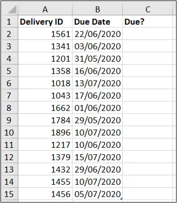
You could write the formula like this;
=IF(B2<TODAY(),"Yes","No")
But this does not take full advantage of the dynamic array engine.
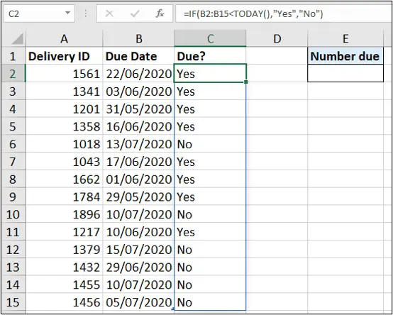
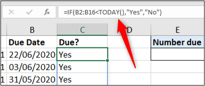
If you write the formula like this;
=IF(B2:B15<TODAY(),"Yes","No")
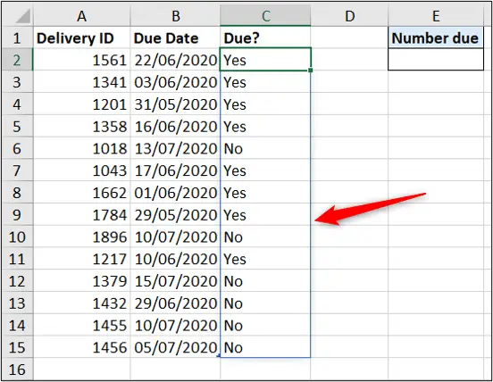
It will automatically spill down the other cells in column C to row 15 because that is where the array B2:B15 ends.
Spill Range and Spill Error
The formula was entered into cell C2 and it spilled down to cell C15.
If you need to edit that formula, you can only do so in cell C2. The other cells do not contain the formula.
From cell C3, in the Formula bar, the formula is visible, but is greyed out and cannot be touched.
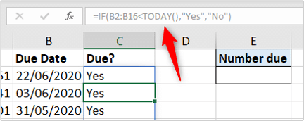
From cell C2, the formula remains active and available for editing.
So, the formula can only be changed from the origin cell.
You may have also noticed that the spill range has a blue border to visually show the array perimeter. This is only shown if you click a cell within the spill range.
If anything was to interfere with the spill range, the #SPILL! error is shown.
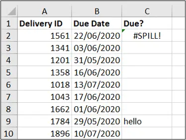
This is fantastic as it makes it easy to notice if any cell in the spill range is affected. It is also easily fixed by removing the interference.
How to Reference the Spill Range
Something else that makes these dynamic array formulas so amazing is that you can reference the spill range.
This means that your formulas are referencing a dynamic range and makes it much easier to create dynamic reports and models in Excel.
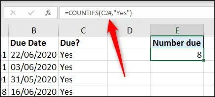
For this example, let’s use a COUNTIFS function in cell E2 to count the number of deliveries that are due.
When referencing a spill range, the hash (#) sign is used after the origin cell address. So for the range argument of COUNTIFS, C2# is entered.
=COUNTIFS(C2#,"Yes")
Often, if you select the range, this is written in for you.
Dynamic Array Formulas and Table Data
The dynamic array examples so far have been used on cell ranges, but these formulas are more reliable when working with data stored in tables.
Tables automatically expand when new rows or columns are added to them so if our formulas use table data, they too will dynamically expand.
This dynamic behaviour is the real game changer behind these formulas.
The data we have been using in the examples so far is now in a table named datesdue.
The following formula would work just like the previous examples.
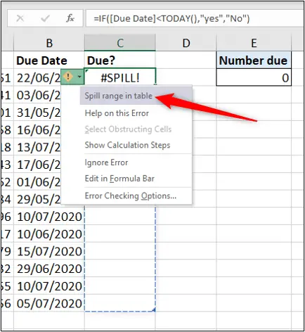
=IF(datesdue[Due Date]<TODAY(),"yes","No")
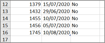
But now we have a true dynamic array because if another delivery was added to row 16, the IF function automatically spills to the added row.
Dynamic Arrays Cannot Be Used in Tables
Unfortunately dynamic array formulas cannot be used within tables.
Tables are for storing raw data whilst dynamic arrays are used for creating dynamic outputs from that data.
If you use a dynamic array within a table the #SPILL! error is produced.
With column C included within the table, we are informed that you cannot spill within a table.
New Dynamic Array Functions
A bunch of new functions have appeared in Excel to take advantage of this dynamic array behaviour.
These include SORT, SORTBY, SEQUENCE, FILTER, UNIQUE and RANDARRAY.
Let’s see an example of the FILTER function in action.
Keeping with the same data, it is now stored in a table named deliveries.
We will use the FILTER function to filter the list and return the deliveries that are due.
The following formula will do this;
=FILTER(deliveries,deliveries[Due Date]<TODAY(),"")
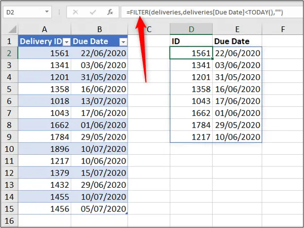
This formula returned an array two columns wide to match the deliveries table which was provided as the array to filter.
You will still need to format cells just like with any formula, so in this example the date cells were formatted in advance.
It is typical to format a larger range than expected as the formulas are dynamic. And if they expand you want to new cells to be readily formatted.
Learn More About the FILTER Function
Dynamic Array Formulas with Other Excel features
Unfortunately, dynamic array formulas cannot be used directly inside Excel features such as Data Validation and Conditional Formatting.
However, you can refer to a spill array from these features. So the dynamic arrays become a stage for the other features to work from.
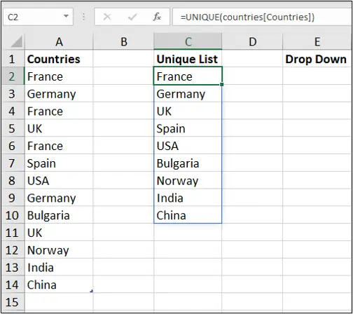
For example, we want to create a Data Validation list from the unique values from this table of countries.
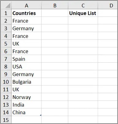
To get a unique list we can use another of the new dynamic array functions named UNIQUE.
The following formula can be used in cell C2.
=UNIQUE(countries[Countries])
As it uses data in a table, if more countries were added, the formula would dynamically expand and accept them. Equally, if countries were removed, the dynamic array would shrink.
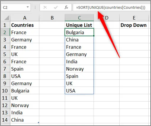
We could take things a step further and add the SORT function to sort the countries in A to Z order.
And then create the Data Validation list from the prepared spill range.
Don’t forget to use the spill reference #.
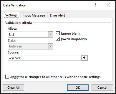
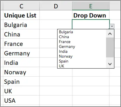
And the Data Validation list is set up.


Leave a Reply