The FILTER function in Excel is a dynamic array function available to Excel 365 users and Excel Online only.
This is an extremely versatile and powerful function – and is possibly the best function in Excel.
It is the formula equivalent of the extremely useful filter feature of Excel. It will return a range dependent upon criteria that you specify.
This range can be returned to a worksheet but also embedded inside other formulas.
The potential for this is huge. With the FILTER function providing the ranges for other formulas, and also our charts and data validation rules etc. This function has changed the game forever.
In this guide, we will introduce you to the FILTER function with different examples. The potential for this function is so vast, that you need to explore it yourself also.
Download the file used in this tutorial to follow along.
Watch the Video
How to Use the FILTER Function in Excel
Let’s take a look at the classic use of the FILTER function. To automatically output a range of data that meet specified conditions.
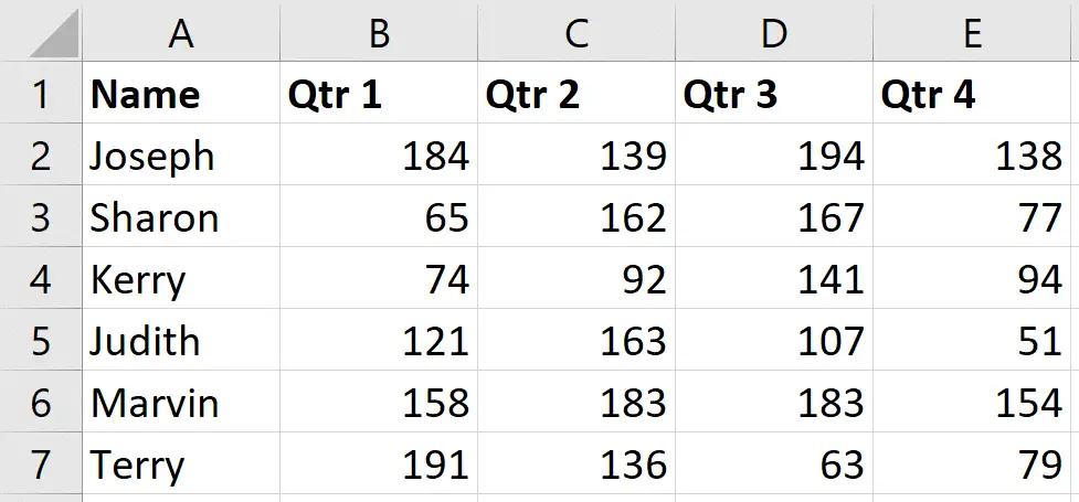
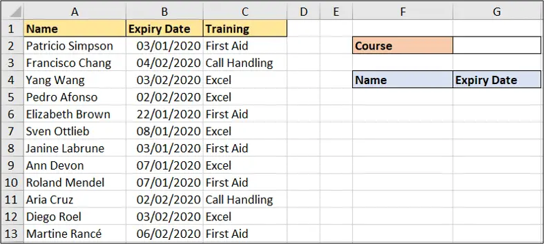
For example, we have a list of training (columns A:C) with a date column for when that training requires renewing. It has been formatted as a table named training.
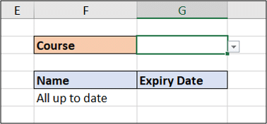
And we want to return a list into the range to the right (columns F and G) of the names and expiry dates of the training that is overdue.
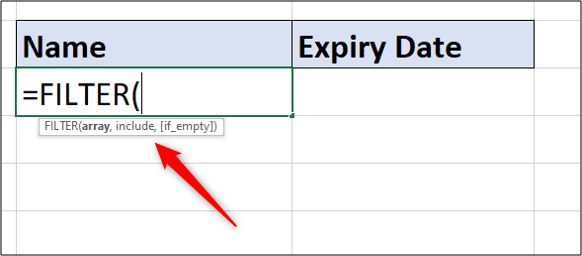
So in cell F5, we will use the FILTER function.
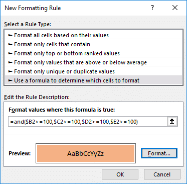
The FILTER function accepts three arguments – array, include and if_empty.
Array: The range of values you want to be filtered.
Include: The filter criteria. Boolean expressions which will determine what rows or columns to return.
If Empty: The action to take if no results are returned by the filter. This is an optional argument.
The following formula can be used to return the name and expiry date.
=FILTER(training[[Name]:[Expiry Date]],training[Expiry Date]<TODAY(),"All up to date")
The Array is the name and expiry date columns of the table (table references are used in the formula) because this is the information we want to be returned.
The following criteria is used for the Include argument.
training[Expiry Date]<TODAY()
This ensures that the expiry date is before today’s date.
Finally the text “All up to date” will be returned if the FILTER function returns no records.
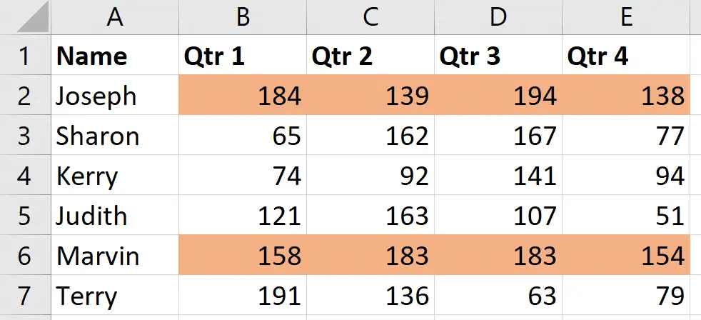
The following results are returned. A blue border is shown around the “spill” array.
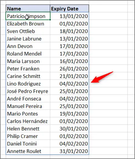
Because dynamic arrays have been used here, all results are returned by one formula. However, to edit the formula, you must do this in the first cell of the array only (cell F5).
Excel FILTER Function with Multiple Criteria
The previous FILTER function example has only one criterion – if the expiry date was in the past.
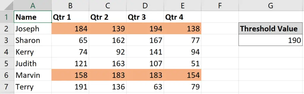
However, let’s test the training course as well. In cell G2 there is a drop-down list for the different courses – call handling, Excel and first aid.
We want the FILTER function to return the name and expiry date of the training that has expired AND for the course listed in cell G2.
To do this we need to surround both logical tests in brackets and multiply them.
This is the complete formula.
=FILTER(training[[Name]:[Expiry Date]],(training[Expiry Date]<TODAY())*(training[Training]=G2),"All up to date")
And here is the Include argument isolated so that it is easier to understand.
(training[Expiry Date]<TODAY())*(training[Training]=G2)
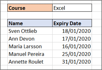
The formula returns the following results when Excel is selected.
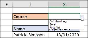
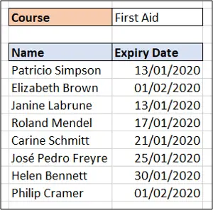
Changing the course in the drop-down would immediately produce the results for that course. Here are the results for First Aid training.
Why multiply them?
Whenever you want to perform And logic and only include the results where all logical tests are equal to true, you must multiply each boolean expression.
The reason for this is because each test is conducted separately.
So all the expiry dates that are previous to today’s date return a true. This is a snapshot of how the first 11 rows of our data are evaluated.
{TRUE;FALSE;FALSE;FALSE;TRUE;TRUE;TRUE;TRUE;TRUE;FALSE;FALSE}
And then all training that is equal to the value in cell G2 return a true.
{FALSE;FALSE;TRUE;TRUE;FALSE;TRUE;FALSE;TRUE;FALSE;FALSE;TRUE}
The two arrays are then multiplied. The rows that are equal to 1 are the results that are returned.
{0;0;0;0;0;1;0;1;0;0;0}
So multiplying the expressions ensures that all tests must equal to True to evaluate to 1.
How about OR logic?
If you wanted a scenario where only one of the logical tests must equal true to be included, then wrap each boolean expression in brackets and add them with the plus operator (+) instead.
Tidy this up with the IF Function
The previous example works great, but only if cell G2 is populated with one of the course names.
If it is not, then the text “All up to date” is returned. And this is not true.
The following formula uses an IF function to test if cell G2 is empty. If it is, then use the FILTER function with no test on a course name, but if it isn’t then use the FILTER function that does test the course name in cell G2.
=IF(G2="",FILTER(training[[Name]:[Expiry Date]],training[Expiry Date]<TODAY(),"All up to date"),FILTER(training[[Name]:[Expiry Date]],(training[Expiry Date]<TODAY())*(training[Training]=G2),"All up to date"))
This formula may seem daunting due to its size. But really it is just two FILTER function being controlled by the IF function and the test on cell G2.
Breaking the formula up onto different lines can make it easier to understand.
=IF(G2="", FILTER(training[[Name]:[Expiry Date]],training[Expiry Date]<TODAY(),"All up to date"), FILTER(training[[Name]:[Expiry Date]],(training[Expiry Date]<TODAY())*(training[Training]=G2),"All up to date"))
Use the FILTER Function with Other Excel Functions
The previous example showed the FILTER function with the IF function.
One of the great advantages of the FILTER function is that it returns an array based on criteria – like a super lookup. And this array could be used in any Excel function.
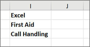
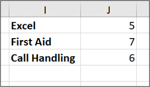
In the range below we will count the number of training that has expired for each course.
To do this we will combine FILTER with the COUNTA function.
FILTER could be combined with any function – SUM, LARGE, VLOOKUP, MEDIAN making it extremely flexible.
The formula below returns the count of expired training for each course.
=COUNTA(FILTER(training[Name],(training[Expiry Date]<TODAY())*(training[Training]=I1)))
The formula returns the names if the date has expired and training is equal to the value of I1. These names are then counted by COUNTA.
The Excel FILTER function is incredibly useful and will change the way people use formulas.
There are so many scenarios where this function will come in handy. For example, below is a video on using it to create a searchable drop-down list.
Some of these special scenarios will become clear as you play around with it and use it in your workplace.