I was asked recently in class how to extract a postcode from an address in the UK. The person asking needed a formula because the spreadsheet updates often and they wanted an automated solution.
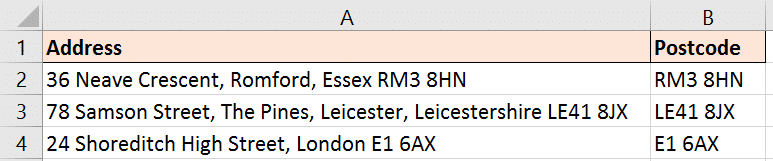
The problem with extracting UK postcodes is that they are highly irregular. They will be at the end of the full address and can come in a different number of characters e.g. E1 6AX, RM3 8HN and LE41 8JX.
They are not as structured as a US zip code may be and harder to extract. Because of this the formula is intense, but I am going to break it down and explain it in detail.
Extract Postcode from Address using an Excel Formula
The formula below is the finished article. If you are not used to writing formulas like this it may seem overwhelming, but we are going to look at it one piece at a time.
To use this formula, simply copy and paste and change the cell references to where your addresses are entered. If you want to know more about how this works, read on.
=RIGHT(SUBSTITUTE(A2," ","*",LEN(A2)-LEN(SUBSTITUTE(A2," ",""))-1),LEN(A2)-FIND("*",SUBSTITUTE(A2," ","*",LEN(A2)-LEN(SUBSTITUTE(A2," ",""))-1)))
How it Works
The RIGHT function has been used to extract the postcode. This function extracts text from the end of a cell. We can be sure that the postcode is at the end, so this function works for us here.
The RIGHT function requires two pieces of information from us. What text to extract the postcode from, and how many characters in the postcode.
=RIGHT(the text to extract from,how many characters)
What we do not know is how many characters are in the postcode of each address. We need Excel to calculate this.
To do so, we will find and mark the start of the postcode in the address. This unique mark can then be used to calculate how many characters in the postcode.
Finding the Start of the Postcode
The postcode always starts after the penultimate space of the address. It does not matter how many spaces are in the address, we can be sure that the postcode begins after the second from last space.
The formula below calculates what number space the penultimate space is. So it basically returns the position of the space.
LEN(A2)-LEN(SUBSTITUTE(A2," ",""))-1)
The LEN function returns the number of characters in a cell. The SUBSTITUTE function finds and replaces each space with nothing, essentially removing them.
Altogether, by subtracting the number of characters in a cell without spaces from how many characters including spaces, gives us how many spaces there are.
The -1 is then used to return the occurrence of the second from last space.
This part of the formula actually occurs twice n the full formula as shown below.
=RIGHT(SUBSTITUTE(A2," ","*",LEN(A2)-LEN(SUBSTITUTE(A2," ",""))-1),LEN(A2)-FIND("*",SUBSTITUTE(A2," ","*",LEN(A2)-LEN(SUBSTITUTE(A2," ",""))-1)))
Uniquely Marking the Postcode in the Address
Now that we have found the postcode we want to insert a unique marker so that Excel knows where it is.
In the formula below the SUBSTITUTE function has been added to the previous formula to add an * at the start of the postcode (the second from last space).
SUBSTITUTE(A2," ","*",LEN(A2)-LEN(SUBSTITUTE(A2," ",""))-1)
This also occurs twice in the formula.
=RIGHT(SUBSTITUTE(A2," ","*",LEN(A2)-LEN(SUBSTITUTE(A2," ",""))-1),LEN(A2)-FIND("*",SUBSTITUTE(A2," ","*",LEN(A2)-LEN(SUBSTITUTE(A2," ",""))-1)))
Calculate the Number of Characters in the Postcode
In the second part of the RIGHT function the formula below has been used to find the position of the * (our unique marker), and subtract that number from the total number of characters in the cell (LEN function). This returns how many characters are in the postcode.
LEN(A2)-FIND("*",SUBSTITUTE(A2," ","*",LEN(A2)-LEN(SUBSTITUTE(A2," ",""))-1))
I do hope this makes sense. It is a complicated formula if you are a beginner.
If you are interested in seriously improving your Excel formula skills. Check out our online course – Excel Formulas Made Easy – Learn over 100 Formulas.


Brilliant thank you.
You’re very welcome.