A Gantt chart is used to plan and track the progress of a project. Although Excel does not contain a Gantt chart feature (maybe one day), its tabular structure and wealth of tools provide us with the means of creating one.
A Gantt chart can be created in many ways to match your requirements.
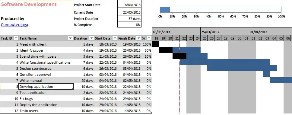
Using the Excel Gantt Chart Template
This Excel Gantt chart template uses fixed scheduling on its tasks and provides a timescale of 1 full year from the project start date. To use the template;
- Enter the project start date in cell E1.
- Enter the ID and name for the tasks of your project.
- Enter the task’s estimate start dates and durations.
- Enter the % completion to update the chart with the progress of the project.
Download the Excel Gantt chart template.
Let’s look at what was used to build this Gantt chart in Excel.
A Thermometer Chart
A thermometer chart has been used at the top of the sheet. This chart is used to visualise the progress of the project easily. It uses the data stored in cell E4 which calculates percentage completion.
Freeze Panes
The freeze panes feature is used to ensure that the project overview section and timescale at the top of the sheet, and also the table of task data to the left are both always visible as you navigate around the sheet.
Conditional Formatting
Conditional Formatting has been used extensively in this Excel Gantt chart template to display the task progress, task % completion, non working days and today’s date.
There are 5 Conditional Formatting rules in total. To view the Conditional Formatting rules;
- Click the Home tab on the Ribbon.
- Click the Conditional Formatting button and select Manage Rules.
- Select This Worksheet from the Show formatting rules for list at the top of the dialog box.
Some of the rules used are quite advanced. Learn more about Conditional Formatting.
- Highlight Saturday and Sunday in a list
- Conditional Formatting with dates – 5 examples (video)
- Conditional Formatting with multiple criteria
Format as a Table
The Format as Table table feature found on the Home tab has been applied to range A6:F18. The table will grow automatically has new tasks are entered into the list. The table is named Entry.
A table is also used on the non working dates on the holidays sheet to automatically change in height if more holidays are added.
WORKDAY Function
The WORKDAY function is used to calculate the date a specified number of working days before or after a specified date.
This function has been used in the Gantt chart to calculate the finish date of each task. Non working days are entered on the Holidays sheet and included in the calculation.
Learn more about how to use the WORKDAY function.


Hi I’ve been working on putting a Gannt chart together and have a basic format put together which works nicely be very happy to share it with you to look over for some advice.
The one you have put together pretty much nails what I’m after however one thing I noticed is that when a task spans over a weekend and you update the completion to 100% the black actual falls 2 days short due to the weekend. Is there a fix to this?
I also wanted to ask whether you had any thoughts on how to change the colour of the acticity to represent different stakeholders. I would like to have say blue for Internal Stakeholders & Red for external is this a possibility?
any help advice or tip would be much appreciated.
thanks
Michael
You could insert an additional column and use it to enter if the task is for an internal or external stakeholder. Conditional Formatting rules can then be created to apply the required colour dependent on the data in that column.
I hope that helps.
As for the completion %, thank you for alerting me to this. I shall have a look, rectify and upload an updated version hopefully within a few days.
It’s actually an easy fix. If we consider that nothing ends or is happening on weekends, just rearrange the cond. formatting of weekends on top of project completion bar.
Visually will represent the truth, and no fix in functionality required.
Thanks! This is an excellent Excel Gantt chart template. I prefer it to others because it is all on the worksheet, and doesn’t use a bar chart for the representation.
However, I also noticed the percent complete does not work across weekends and holidays. The problem is simply that the conditional formatting formula is only counting the duration days for the task and not counting the weekends and holidays. I fixed this by changing the first conditional format formula, substituting the difference in finish date and start date (E-D) (that compensates for weekends and holidays) for the number duration days (C).
So, instead of AND(G$6=$D7,($C7*$F7)>=1), use AND(G$6=$D7,(($E7-$D7)*$F7)>=1). Works like a charm!
Hi Mike,
Thanks for your awesome formula.
The formatting was intended to only count the working/billable days though.
Gantt charts can be used in many ways to accommodate the way in which that project or business operates. It is good to know how it can be adapted to meet certain requirements.
hi, I need help, as I would like to remove the weekends as non working days, please do render ur kind assistance as the method u stated in the comment did not work for me. Would need it for a project so it’s kind of urgent, your help would be much appreciated. Much thanks in advance
GENIUS!!! This is the awesomest spreadsheet I’ve seen in my life!!! 😀
Thanks for this!
What is the simplest was to remove the grey blocks that exclude weekends and holidays?? I know nothing about excel so the most simplest explanation would be highly appreciated!
Thanks you!!
Should be able to remove the columns manually.
I’ve downloaded your worksheet and is realy an awesome work.
May be it should be an update because:
“There are 5 Conditional Formatting rules in total…”
I just have 4 and the black progress bar is not working.
Can you please share the link for the latest template reflecting the % complete gantt chart, or else please explain the rule for % complete conditional formatting.
Thanks,
Rafael.
Hi Rafael, the link can be found in the post.
Hi,
Sorry, but I’ve downloaded again from the post link:
Download the Excel Gantt chart template.
And the % of completion is still not working.
Do you have another link?
Thanks.
Hi Rafael,
I just checked it and it downloaded fine for me. Enter values in the % complete column and if the % is big enough to warrant and update a black bar will display the progress on the chart.
I am sorry you are having issues with this but the link works fine.
Alan
Just a line to thank you for sharing this 🙂
i.
hi there.
I have a few basic questions. how do i change this so that monday is the first day of the week?
Also why does it add so many days to the chart. i.e. i say 5 days and it adds them as 7 on sum row and 8 on others? Is it possible to high light certain tasks in a custome colour? is it possible to add a box that says how many tasks are to be completed that week?
Sorry i know this is alot of questions but i really am the most basic of users and find this sheet be very useful for what i need.
many thanks
Hi Geoff, although these kind of things can be set up they are not incorporated in this Gantt Chart.
Conditional Formatting rules would need setting up for the Customer Colour. A formula at the top for how many that week. As for the number of days. The days you enter are working days, the Gantt Chart displays calendar days so excludes weekends and bank holidays.
Hi and thank you for your gantt chart.
I’m new to all this and have used the template to chart the progress of a new project.
in the left hand window i have 24 tasks but only the original 12 from the template are updating in the timeline on the right hand window…
How do i include the other 12?
Hi again, just managed to get the other rows to work…however now after the third row of the right hand window it seems to have skipped entry 4 on the right window. it now seems to show the timeline value for the window on the left on the row above!! HELP!!
Sorry Jono, I’m not sure what you mean. If new tasks are added to the bottom the table on the left show expand automatically. The chart on the right can be copy and pasted manually.
How to add task & keep track of progress..I can add task but cant see chart against it.
Hi Hitesh,
To add new tasks, enter the on the next empty row and copy and paste the chart side manually.
Alan! Awesome template… I’ve been looking around for a while and this one really nails it to my taste… Simple enough to maintain, good looking — THANK YOU! I’ve already expanded on it to better suit my needs and am very grateful to you to have gotten me started on the right foot!
May I ping you with a couple of questions though: what is the difference between “nonworking” and “holidays”. They both echo the same range of cells, albeit one is the name of the Table and the other is a defined name.
Also, I’m not sure I get how the “greying” Conditional Formatting of the week-end & holidays formula work out. Specifically, the last argument of the formula that applies to greying a holiday in: =OR(WEEKDAY(G$7,2)=6,WEEKDAY(G$7,2)=7,G$7=holidays).
If you copy/paste this into a cell, with a valid reference to a holiday, you get “FALSE” as a result; the only way to get “TRUE” out of it is to use an array formula, e.g. using the “{” “}” signs in the formula, as “holidays” refers to a range of multiple cells. Do conditional formatting formulas work by default in array style?
Again, many thanks for this and I wish you and your family a very Merry Christmas and all the best in the New Year.
Cheers!
–Alain
Thank you Alain for your kind words. In answer to your questions;
With the defined name and the table. This is done to make the defined name (holidays) dynamic. I need it to grow automatically if new dates are entered in the list so that the Conditional Formatting rules automatically pick these up.
Now there are other ways of achieving this so a Table and defined name is not necessarily the way to go, but it gets the job done.
With the Conditional Formatting rule, they must do. Aslong as we have our mixed reference in there (G$7). CF knows to check the dates of that task for that row only. It is kind of the direction of travel as it compares the criteria.
Can u pls guide us how to create such gantt chart in excel.
Hi Alan,
Request to guide me to prepare similar gantt chart as i am finding difficult to produce such report.
I am looking/using this Gantt chart for the first time. First look says that it is just what I have been looking for. So far, I am also having trouble getting the link to give the updated file to include the correction for the % complete conditional formatting. My copy of the chart only has four rules. I have added a new rule, but I have not yet worked out the kinks. I have “Use a formula to determine which cells to format” Rule Style selected. This is what I have inserted for the “FORMAT VALUES WHERE THIS FORMULA IS TRUE”:
=AND(G$6=$D7,(($E7-$D7)*$F7)>=1).
I am also having trouble with the thermometer percentage bar. Even when I give the % complete cells(F column) all 100%, the thermometer bar only goes to just under 60%.
Thanks in advance.
Hi Rick,
I cannot understand why it is not working for you. I just downloaded the one from the webpage and tested it and it all works fine. Both the CF rules and the thermometer chart. I have re-uploaded it to the server again.
Drop me an email if you have any other problems. I’ll send you it.
Alan
I am sorry to be such a bother, but I have tried downloading it again and there is only the four CF rules. Maybe it is because I am running Excel 2007? Please try sending a copy to my email address.
Thank you for your help.
Rick
Hi Alan,
I started using this Gant chart but whenever i am putting task date (Start & Finish) & completion % than Chart showing in another column (goes one cell down). instead of showing in same column bar.
Kindly let me know what might be wrong in that!!
Hi Vrijesh, its hard to say without seeing a file. Maybe just try downloading the file again and re-inputting your tasknames and dates.
First of all, THANK YOU for such a terrific template. It’s just what I was looking for.
Second, I’m having some troubles with the CF. I mean, the first row (the task number 1), works alright, but the other ones are not painted with colors when I change de number of days or so. Have any idea about what’s going on?
Thanks again !!!
Hi Marisa,
Thank you for your comments. I couldn’t say what your problem is without seeing the file.
The % complete formatting does not work on versions before 2010 as it references another sheet, but the duration should be fine.
Hi Alan,
Thanks for the Gantt chart.
Question: how do i change that the weekend days are counted as working days?
thanks again!
Lucas, I have dropped you an email.
Hi, care to share the solution? I want to include Saturday but not Sunday.. need this urgently. Thanks!
The Conditional Formatting can be done easily as the Weekday function has been used to format cells based on day of the week for non-working days.
For % complete, because the Workday function has been used to skip weekends. To only miss one of the days you will need to list all the Sundays throughout the lifetime of the Project to specifically miss only them.
Hello Vrijesh, Thank you for this gnatt chart. I’ve been trying to find one as learning tool and this is perfect. Can you please tell me what the different colors in the chart mean under conditional formatting? I figured out the blue one means if the task is not 100% complete the bar is blue. But what does the red vertical red line mean and what does it mean when the pink fushica color appears in the middle of the bar? Thanks again!!!
Hi Joi, Thank you for your comments. The name is Alan though 🙂
The red line indicates today’s date in the schedule. The line on the blue bar is todays date shown when a task is present on that date. Grey is non-working days such as weekends and holidays. The black is task progress when the % complete column is updated.
Thanks for the free download, Gantt chart is really what I was looking for, but because am not skilled enough in Excel and in simple words, how would i change non working days to be Fridays and Saturdays instead of Saturdays and Sundays.
Appreciate your help.
Thanks
Hi Walaa,
For the Conditional Formatting part of the chart the WEEKDAY function can be used to identfy any day of the week. As for the Finish Date of a task, it would probably be easier just to enter it, otherwise we could make calculate a finish date using the NETWORKDAYS.INTL function with a formula.
I get alot of requests on this blog post so am hoping to release a course soon or some other kind of project management in Excel training.
Alan
Hi Alan
Great Gantt Chart template. Have you uploaded a more recent version following previous comments that the % is not showing in black?
Downloaded the template yesterday and it shows Task 1 as 100% complete in blue not black?
Can you help please.
Hi,
The template progress will only work from Excel 2010+ as the Conditional Formatting references a different worksheet (Calculations). This data can be moved and the CF rules edited to work in previous versions.
Alan
Awesome template, I am running 2007 and was wondering if you could give a little insight or a formula to allow us working in the stone age to get the progress bars to turn black with the percentage cells. any help is greatly appreciated. Thanks, Ron
Hi Ron,
The problem here is that the formula references the little table showing completed tasks on the Calculations sheet. You were only able to reference different sheets from within Conditional Formatting from 2010 (what took them so long??).
For it to work you will need to cut and paste the table to somewhere on the same sheet (stick it right out the way if you don’t want it visible). Then edit the CF rule for the black bar to reference that cell rather than Calculations!B7.
Hi Alan,
Thanks for this great template. Is there any way so that we can extend it for 2 years.
Absolutely. You should be able to copy the dates and the formatting across for as many weeks as you need.
Hi, i would like to ask why i am unable to open the template?
I have no idea Bryan. It is just an Excel file and should open like any other.
Hi Alan, thanks so much for the chart, it is really going to help me out with my project.
I’ve modified it to the needs of my project, but one thing I can’t seem to be able to do is include the weekends as working days. E.g. for one one of my tasks i entered 14 days, but it is showing as 20 on the Gantt chart. From what I understand I need to change something to do with the ‘Conditional Formatting Rules’, right? Would it be possible for you to help me with what it is that i need to change, as I’m struggling to understand how the ‘rules’ work and what they mean.
Hi Tomi,
When you look at the Conditional Formatting rules, you want to delete the grey one. This will remove the highlights for non-working days however it wont affect the calculations.
You will also need to go to the Calculations tab and just add the days on top instead of the WORKDAY function that is there.
Hi Alan, Thank you very much for the gantt chart.
Can I ask what does the conditional formatting -> =AND(G$6=$E$2,G$6>=$D7,G$6<$E7) try to do?
Thank you.
Hi Alvina,
Sure that rule is used to display todays date on the Gantt Chart with a dashed red line.
Hi Alan,
Thank you very much. That clarifies my doubts.
If I like to highlight the whole duration of the project with another colour and also the ongoing tasks with the current colour, could you advise the rule to be added in the Conditional Formatting?
Thank you once again.
Hi Alan thank you for this template. Couple of questions, looks like some formatting is missing from the template when I down load it. The bar don’t change color based on percentage complete. Looks like one of your conditional formatting formulas is missing. Can you please verify and correct or email me a copy with that in it. Secondly I have several projects with many tasks and due dates, is there a way to give each project a tab and have a master tab that has all the tasks and can sort them by due date so I can work on all tasks from one tab? Thanks, cheers!
Hi Jay,
Sounds like you have an Excel version prior to 2010. The formatting for the % complete references a couple of cells on a different sheet (the calculations one). Excel could not do this without using a Range Name or something prior to the 2010 version. You will need to copy and paste the data from Calculations to somewhere on the same sheet and modify the formatting references.
As for the multiple projects. Almost anything can be done. First thought is that a macro would be best due to the intensity of the work. Formulas can be used such as VLOOKUP to link it up, my only thoughts are that if there are alot of task this may weigh heavily on the file and slow it down.
Alan
Hi Alan,
Thank you very much ! :), your guide is very useful for me.
I usually work online with our team members. So i have put your template to google driver and open it by googlesheet on web, some function doesn’t work: – Black colour % finish is don’t change colour.
– Add more row is not automatic by type some charactor in new row.
I have try to change something in function but can not solve this problem.
Can you help us to have version for googlesheet?
Thank you very much !
Binh
Hi Binh,
I don’t have a Google version of the Gantt Chart. Maybe some time in the future.
Alan
Hi Alan
I’m having trouble with the percentage completion formatting. I added new rows and copied the formatting down (columns A-G, from row 12), but the conditional formatting on the right didn’t come up once I’d carried on populating duration, dates, completion, etc.
I tried using format painter, which did recognise the start & duration data, but then it didn’t recognise percentage complete and kept the cells blue (not changed to black).
Any ideas what I’ve done wrong? I’m using Excel 2010.
Thanks
Hi Polly,
The percentage complete uses data from the Calculations sheet also. You may need to check the data here. If you added additional rows to the table, the data here may need copying down for each new row you added.
Alan
Hi mate,
Great spreadsheet, you are doing great work!
I have amended the chart slightly and have included an extra column to assign each task to a department. I’m sure there is a way to use conditional formatting to colour code the tasks based on departments but my excel skills are not strong and I am struggling to work it out. Could you possibly show me how to do this. Fyi, I have six different departments.
Cheers
Hi Ads,
Sounds good. You would need to add 12 new Conditional Formatting rules if you want to keep the red dashed todays date indicator. 2 rules for each department.
Click anywhere in the area of the task bars and then click the Conditional Formatting button and Manage Conditional Formatting Rules. They would be added here between the black one and the blue ones. Each rule would just be a slight enhancement on the previous rules.
For example the current formula for standard blue bar indicator is;
=AND(G$6=$E$2,G$6>=$D7,G$6<$E7) This would be updated to the below if you are recording your department in column C and you were checking for the Accounts department. =AND(G$6>=$D7,G$6<$E7,C$6="Accounts") Hope this helps Alan
Hi Alan,
Thanks for this sheet it is great. Although I am having trouble implementing the formula above. Do I delete the blue ones completely?
I’m sorry I don’t understand your question.
Thank you so much for the template! I tweaked it to work for a schedule with a gantt chart by month/year instead of day/month. Being able to see how you used your conditional formatting was super helpful!! No more banging my head against excel charts 🙂
Hi,
how did you turn DAYS into MONTHS?
Thanks,
Erik
Hi Erik,
Quite a few changes would need to be made. Row 6 will need editing from days to months. The MONTH function can help with this.
But then the formulas calculating duration and the Conditional Formatting would all need changing as they work with days. This is not a small task.
Hi!
Great template!
I have redone the template quite mutch to use it in my work and now I have lost the red dached line that indicates todays date.
I really would like to have this line, how do I do from start to end to get the line with Conditional Format for the hole excel document, I have tried but I can’t get the dached line back.
Thanks for your help!
Thanks Lis.
If you download the original file, click on any cell in the chart area and then click Conditional Formatting and Manage Rules.
You will see two rules are used to create the dashed line. One at bottom of the list of rules to create dashed line on cells with no activity and another second from the top to create the dashed line aswell as the blue task bar.
Select each in turn and click Edit Rule to see the formula and adapt for your redone template. The formatting itself you can change if necessary. I just did a red dashed line as left hand border.
Thanks! Now it worked! 🙂
Hello!!
Thank you for this chart, it is almost exactly what i would need. One thing I would like to change but cannot seem to figure out for myself is the Gantt Chart view. Your template is set so that you can see individual days, is there a way to roll this up so that I see the information in weeks or months? My project goes until 2016 and would like to show a higher level view.
Thanks so much!
Hi Niedra,
I don’t have a Gantt Chart spreadsheet using a higher level timeline. I’m sure it can be done but think alot of the formulas and CF rules would need to be re-written.
Hi,
thank you for this great template!
I have just one question. How can I change this so that Monday is the first day of the week even if the project start is maybe on Wednesday?
Thanks
I’m not sure how this makes a difference to the chart. Do you mean Monday as a non-working day?
Dear,
I faced the same problem related with 5 Conditional Formatting rules in total. After downloading the excel file, i just could see 4, can you kindly share the code utilized for progress bar that is in black color?
Thanks in advance
This is the formula for the progress bar. It will only work in Excel 2010+=$D7,Calculations!$A$7>=1)
=AND(G$6
Hi, thanks for the awesome template. I was wondering that how I can add ‘Dependency’ column in order to create dependency between multiple tasks.
Thanks,
Thanks Farrukh. Yes you can do that. Link the task to the finish date of the predecessor with +1. Or use the WORKDAY function for the next working day after the predecessor.
can i add another task?
Absolutely. Add it to a new row and copy the formulas and formatting down.
Hello,
Thanks for this. I am very pleased to get this. Thanks once again.
I have fall a problem. can you help me please? Which I can not increase the completed working area that should be colored in Black. What should the formula for this? please help. i have attempted many time.
thanking
Riaz
Bangladesh
The progress does not work in Excel versions prior to Excel 2010 because it references data on a different sheet.
If you use a version prior to 2010, copy the table from the Calculations tab and paste it somewhere on the Gantt Chart sheet so it does not affect the Gantt Chart.
The formula for the progress Conditional rule is;
=AND(G$6=$D7,Calculations!$A$7>=1)
Create a CF rule and adapt this formula so it works on the data you hve copied across. Make this rule the top of the 5 in the CF list.
Hi – like a few others, I’m still struggling to move the calculations formulas to the Gantt sheet and have the black line update. I can’t work out how the formulas are working in the calculations sheet and how to update them once moved. Can you offer any advice please? Thanks
Just as an update I’ve got the numbers matching what the formulas were in the Calcs tab, but the CF only makes the 1st cell of each row black, not the actual percentage it should be. Just can’t work out why!
Hi Darren,
This link will allow you to download a version with the progress bar included. This is for versions prior to 2010.
The data used from row 21 can be hidden.
Hello,
How can this Gantt chart template generate network path
It does not provide a Network Path view.
Alan
many thx for supply such a valuable resource. I’m using thiss template to plan multiple projects & respective tasks. Am keen to extend the range of dates to end 2017 – what is best way to insert ?
You can copy the dates across to extend to 2017. The chart is set up as days however so the chart will be large. How might want to check out how they are set up and use weeks if your timeline is that large.
He visto tu sitio y me semeja de lo más interesante.
No solo por el hecho de que lo que estás planteando tiene un amplio
conocimiento (o por lo menos eso aparenta) sino más bien que la forma que cuentas con de expresar
tus ideas es genial. Espero que en algún instante podamos trabajar algo juntos o al menos que me des la
oportunidad de percibir alguna visita tuya a
mi blog y me des tus puntos de vista. Al final del día quien sino más bien otro blogger para
juzgar el trabajo de uno.
generalmente no comparto comentarios porque me da pereza ingresar y todo eso,
pero esta vez vi algo que me ha hecho pensar un mensaje para darte
las gracias por tu trabajo. este comentario no
ofrezca mucho a los otros lectores pero espero que aporte un apoyo para
que la blog continue creciendo semana tras semana hasta que sea la numero
uno de internet
many thans for this amazing template. Is going to be a huge contribution for many projets. But, I have one doub, when I add more task to the template, and change the percentaje, the color of the cell dont change. Can you explain why this could be happening please?
You need to copy the cells containing the formatting down
How do I remove the workday conditional formatting? I’d like to account for all days in the percentage complete.
Hi Patricia,
The can view the Conditional Formatting rules and the percentage complete should be the top one. However I think the problems is more to do with the WORKDAY function used on the Calculations sheet.
Alan
Amazing spreadsheet. Salute!!
Hi, very nice and usefull thanks for sharing
it will helps a lot,
don´t you have similar template not for days but for weeks?
I tried to do it but it is quiet difficult for me…
thanks a lot
Amazing spreadsheet, but I do have one question regarding the older excel version. The duration complete on the first page cannot be lowered to allow for new tasks to be added, is there a way to move this formatting so the percentage of completion still shows on the task bars?
I’m not exactly sure what you mean David. However if you are using a pre-2010 version the data on the other sheet needs to be on the same sheet as the Gantt Chart. The Conditional Formatting will then need tweaking so that it does not continue to look on the other sheet.
Hi Alan,
I absolutely love the spreadsheet. Is it possible to post another link to the same spreadsheet, but mapping month/year instead of day/month, which would show me more of my schedule in one view, since I need to spread over 2 years. I don’t understand all the different calculations yet in order to get the mapping correct. This would be so appreciated. Thanks.
Regards
Rich
I would love to get some alternative versions of the Gantt Chart together at some point in the future. Not sure when this could be though.
Thanks for the comments Rich.
Hi Alan,
That will be great if at some point that you could share some alternative versions. I will stop by the site once and awhile to check. Thanks again for sharing what you already have !!
Regards
Rich
Hi Alan,
This is great!!! One question.
I want to be able to enter data on top of the date bars (say, to note an event that happened on that day), but i want that info to sort when i sort the data columns on the left hand side. How can I go about doing this?
I have no idea.
do you know if it is even possible? it is the final piece of. big project I am working on. or could you point me in the direction where I may be able to find the response?
I am sure it is possible. In MS Project in would be simple. We would need a clever trick to get it working in this Gantt Chart. I am sure possible though
There are no resources I know of on this. There are very few Excel Gantt Chart I have seen at the level of this one.
thank you sir!
Great gantt chart Alan, it only displays in full days, how do you change the cell format if you want to add non-full days? ie 0.25, 0.5, 3.5 etc? So it would then display 0.25 days?
Thanks,
Darran
We would need to change the Conditional Formatting and formulas also. Its a big job and I don’t have a template for it unfortunately.
Great gant chart!
The reason the % complete does not work in the following scenario. If the duration is 2 days but the work is spread out of couple of weeks (start date and end date) than the % complete does not work. So the the duration needs to be the same number of days as the difference between the start date and end date.
In project this is often not the case. Do not know how to fix this. Do you have a solution for this?
Thanks for your response.
Kind regards,
Sander
Thanks Sander, this Gantt Chart template does not reflect actuals against a baseline so does not provide the capability for the entering of actual start and end dates. I am hoping to one day create a better template including this technique and others.
Hi Alan
Awesome Gantt template. Truly great. I am having a problem though. Why do the the bars lose their CF when you zero out the very first task on row seven? I thought it was something I was doing wrong, but I re-downloaded the template and it still does it. Is there a relationship between the very first task and the ones that follow it? Sort of like predecessors.
In short, if I add days and percent complete to all the tasks, and then put a zero in cell F7, the rest of the rows lose their CF.
Any ideas?
Regards and great work!
Mike
Hi Alan
This template is out of this world good! Thanks! One question. Are the tasks from row 8 down connected to row 7 in some way? If all the tasks below row 7 have a % complete assigned, and then you zero out row 7, it removes the CF from the rows below. Almost like there is a dependency there.
Any ideas?
Mike
Thanks Mike, I appreciate it.
There are no predecessors between the task so row 7 should not affect the others. I just had a quick look myself and entered 0 for the duration of row 7 and it still works fine for the others. Only the row7 bar disappeared.
I’m not sure what may be going wrong.
Hi Alan
Thanks for the reply. Not sure what is doing it. I am using MS Office 2010 if that helps. I downloaded your template again so I had a clean copy, and it happened on that one too. I just can’t pinpoint why it is doing that. Very strange if you ask me.
I have input varying data for Duration and Percent Complete for each of the 12 original tasks. Once they are all filled in, if I either zero out the Duration or zero out the % Complete data from row 7, all the CF’s for % Complete for everything below it gets removed. I am really perplexed. I’d love to send you sample data if possible.
Thanks
Mike
You can send a copy of the file you are having problems with to [email protected] and I’ll try to have a quick look.
Hi Alan,
Love this template, you have saved my life!
I am having an issue with the calcs sheet, I have added another 50 or so tasks, but can’t get the calculations sheet to work, have just copied the rows down but it is showing #VALUE! error… Any ideas?
life saver, thank you for template
I would like to change the Gantt bars to different colors to represent certain tasks or categories. Can you please tell me where I can change from blue to other colors? (Great tool. THX.)
Thanks Paolo. You would need to create a column in the table for the category name and then edit the Conditional Formatting rules for the charts to apply the relevant colour. The rule(s) that you add will need to be above the blue bars in the Conditional Formatting list, but no the black ones or you will lose the progress update.
Thanks so much for the great template. After searching, this is such an easy one to use, great and simple 🙂
Just a question, so i am putting in a start date of say 1/06/16 and the end date is 2/06/16 as an example (1st – 2nd of June, 2016), it calculates this as 1 day on the gantt chart colour, but my problem is that i would like it to be inclusive of both dates. I.e., to say 2 days and also colour in 2 days (those dates mentioned), because the 1st is one day and the 2nd is also another day. We have lots of trainings that are two days for example, but when i put in say 5/7/16 – 6/7/16 it prints the colour out as only 1 day… that being the first day (5th)… Is there a way to change this with a +1 somewhere? Where can i find the area to change this function / where are the formulas for this?
If not, no probs, thanks anyway for the chart, i’ll still use it
thanks so much
The bars are controlled by Conditional Formatting. You can find these rules by clicking in the chart side of the template and clicking Home > Conditional Formatting > Manage Rules.
There are a few in here. But if you check them out, you will be able to add a +1 in there.
To view the gantt chart by week rather than day as earlier suggestions, presumably all you have to do is hide days 2-7? I’ve just downloadsand it seems to work? Great spreadsheet – thanks
Thanks Paul. Yes you could do that. Depends how accurately you need it all to work, but that would offer a higher overview rather than days.
Hi Alan,
Thank you so much for the nice file. I have a question. I seem to not be able to delete a row. When I delete a row(highlighting the whole row, right click and delete) my whole Gantt Chart messes up, all the conditional formatting in Gant Chartt area get affected when I delete a row. Could you advice for a solution to delete an existing row without problem? Thank you.
Hi Sara, sorry but I do not know why this would be. I just tested it and it works fine. All I can suggest is checking the Conditional Formatting ranges and formulas to see what they are doing.
Hi Alan, this is a great tool. Exactly that what I need and which I will use in the future.
but the % (in black) doesn`t work fine when I am adding new Actions (new lines).
Can you send me the latest Version of the Excel sheet please?
Thank you!
I love this Gantt chart, but each time I add a new task, the chart on the right does not fill with black when I put a percentage complete in.
What am I doing wrong?
Thanks Tony. You may need to copy the formatting on the right down for the extra rows, and then on the Calculations sheet copy those formulas down for the rows(s) you have added.
Got it, Thanks!
Hello,
% is not reflecting in the bar. could you please tell conditional formula for that?
Hi Vinay,
It may be because you are using a version of Excel previous to 2010. In these versions Conditional Formatting could not work across worksheets without using named ranges or VBA.
Download this copy where the information from the calculations sheet is on the same as the Gantt ensuring it works in older versions.
Excel Gantt Chart 97-2007
Alan
Hi Alan – I have been using this for a little while now and is an excellent tool. It is much better than some of the histogram charts often found on the net. I have wrestled with Project 2010 for a number of years and found it to be too cumbersome (if not buggy) so have decided to use your chart instead. I have added some minor changes such as differentiating between holidays and non-working days. I would like to add a recurring task function for rolling projects but am struggling with that one ! Any ideas ?
Kevin
A recurring task could be added as individual tasks. Lets assume they recur every Friday. You could enter the first 2 Fridays into different cells one below the other. Select them both and then copy/fill them down to as many cells as necessary to generate the recurrence pattern. The chart on the right can then run of these.
To make it like Project (if you want) you could select the recurring tasks and group them using the button on Data. This will look a bit like Project and their recurring tasks.
Hi Alan – Yes that works well and it looks a little like project too! I didn’t want dozens of identical tasks so this is a good way to hide them.
Awesome, good work Kevin.
Hi how do you get the chart to show more than a year?
If you select the cell on the end of the Gantt Chart and fill/drag them across to the right, it should work. Include the weeks, days and formatted cells in your copy across.
File not found error !!!
This has now been fixed.
Hello Alan,
I hope you are doing well today.
BIG THANK YOU FOR CREATING THIS AWESOME CHART. It has everything needed for tracking progress on a project. You’ve saved me a lot of time 🙂
Thanks again and have a wonderful day!
Best Regards,
Metodiy
You’re welcome, Metodiy. Thank you.
Hello Alan,
May I ask you for quick assistance. I have a new project for which we have as a requirement to have only calendar days (weekends and holidays to be calculated in the project duration). I believe you’ve already gave an answer in this threat but I didn’t get it.
“”””Tomi says
11 June 2014 at 11:29 pm
Hi Alan, thanks so much for the chart, it is really going to help me out with my project.
I’ve modified it to the needs of my project, but one thing I can’t seem to be able to do is include the weekends as working days. E.g. for one one of my tasks i entered 14 days, but it is showing as 20 on the Gantt chart. From what I understand I need to change something to do with the ‘Conditional Formatting Rules’, right? Would it be possible for you to help me with what it is that i need to change, as I’m struggling to understand how the ‘rules’ work and what they mean.
Reply
computergaga_blog says
13 June 2014 at 7:13 am
Hi Tomi,
When you look at the Conditional Formatting rules, you want to delete the grey one. This will remove the highlights for non-working days however it wont affect the calculations.
You will also need to go to the Calculations tab and just add the days on top instead of the WORKDAY function that is there.”””””
I understood the first part about the conditional formatting. But not this – “just add the days on top instead of the WORKDAY function that is there”.
Could you please elaborate, how exactly I need to change the formula.
Once again, thank you very much!
Hi, this is an old post so I don’t remember the rules exactly. The WORKDAY function however is used to calculate a date in the future, that is a specified number of working days only.
Because in this example, you want to include all days, and not just working days. Then you can just add the task duration days on top and not use WORKDAY.
Hi Alan,
Thank you for your answer. I’ve tried this already to add a formula “=Date + total task duration” but then the conditional formatting doesn’t work properly. Could you propose a workaround?
Thank you.
Best Regards,
Meto
That should calculate the end dates for the tasks. not sure on the CF issue.
I would need to open the spreadsheet and look through the rules again, This blog post is years old.
Hi Alan,
I believe I fixed it but thank you again for being so responsive. This is the formula I now use and it seems to work =[@[Start Date]]+[@Duration]
Best Regards,
Meto
Excellent! Nice one!
Hello,
Thank you for this. Very helpful.
Can you please share google sheet link of the same?
Some formulas are showing error when uploaded to sheets so.
I don’t use Google Sheets. Sorry.