The Conditional Formatting tool can be used for some very cool tricks in Excel. Today, I needed it to format all the Saturdays and Sundays in a list.
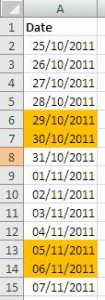
A user had a list of dates and she wanted to highlight each Saturday and Sunday in the list so that they would be instantly recognisable. It also creates and nice effect by splitting each week into blocks.
Create the Conditional Formatting Rule
- Select the cells containing the dates
- Click the Conditional Formatting button on the Home tab
- Click New Rule in the list
- Select Use a formula to determine which cells to format from the top half of the window
- In the Format values where this formula is true box, enter the formula below
=OR(WEEKDAY(A2,2)=6,WEEKDAY(A2,2)=7)
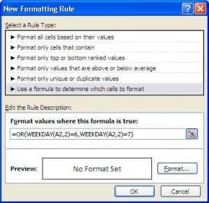
- Click the Format button and select the formatting you want to use to identify the weekend days
- Click Ok
Understanding the Formula
The OR function is used to test the two conditions and evaluate the answer to true or false. The two conditions are:
- Is this date a Saturday – WEEKDAY(A2,2)=6
- Is this date a Sunday – WEEKDAY(A2,2)=7
The WEEKDAY function is used to return the number that represents the day of the week for a date. The Weekday function requires two items of information.
Serial Number – The date you want to return the day of the week for. Cell A2 was used in the formula above
Return Type – A number that determines what day of the week a week begins. Number 2 was used in the formula above to determine that a week begins on a Monday and ends on a Sunday. Therefore Saturday is the sixth day and Sunday is the seventh of the week.


that is great, I did not know this could be achieved, it is very useful.
Sir, 25th Sept.2020.
Very clearly you have shown the topic,which is very easy to understand.
Hoping to receive more ideas in near future too.
Thanking you very much for taking efforts.
Kanhaiyalal Newaskar.