• Skip to main content
  • Skip to primary sidebar
  • Skip to footer

Microsoft Excel Tips and Tricks - Computergaga

  • Home
  • Excel Online Courses
  • Excel Functions List
  • Free Downloads
  • Blog
  • Tutorials
  • About
Home / Archives for Formulas

Create a Case Sensitive Lookup Formula in Excel

Excel lookup functions such as VLOOKUP and MATCH are not case sensitive. They will not worry about matching the case of the lookup value and the cell entries when they search.

But what if you need the cases to match? Well let’s have a look.

Ensuring an Exact Match in the Lookup

To ensure we have an exact match we can use the EXACT function. This function compares two strings of text to see if they are the same, and if they are it returns TRUE, but if they are different it will return FALSE.

The EXACT function looks like this;

=EXACT(text1, text2)

Text1 and Text2 represent the two text strings that you want to compare. In our example these will be the lookup value, and the range of cells we are looking in.

Because we are going to be asking the EXACT function to test one piece of text against a range of text entries, our lookup formula will be entered as an array formula. This special type of formula is entered by pressing Ctrl + Shift + Enter, instead of just Enter and are sometimes referred to as CSE formulas.

Create a Lookup Function with Exact Match

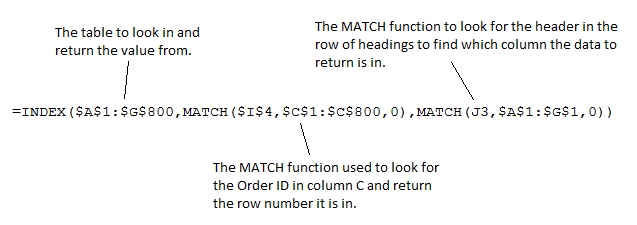
The INDEX and MATCH functions will be used for the lookup in this example. These two functions offer a very versatile Excel lookup formula. If you use functions like VLOOKUP on your spreadsheets and are not familiar with these, I suggest checking them out. You will not be disappointed (Learn more about INDEX and MATCH)

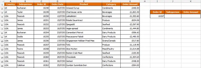
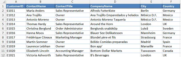
In the example below, we want to return the city that a customer is based in from a list using the customer ID. We want to force the customer ID to be entered using the correct case.

Use Excel lookup function on customer list

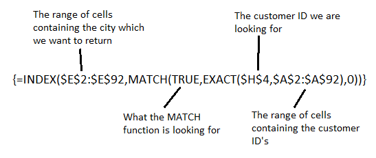
The Excel lookup formula below is used to create a case sensitive lookup for an ID entered in cell H4.

Case sensitive lookup formula using INDEX, MATCH and EXACT

You do not type the curly braces when writing the formula. Excel will input these when you press Ctrl + Shift+Enter.

The MATCH function is looking for the value of TRUE. This is because the EXACT function has been used to test the customer ID against all the ID’s in column A. The value TRUE is returned if an exact match is found.

Watch the Video – Case Sensitive Lookup Formula

Multiple Condition Lookup Formula in Excel

You may require a multiple condition lookup formula in Excel to perform a lookup based on the values in multiple columns. For example, in the image below the formula in cell B3 returns the code based on the country and area specified in cells B1 and B2.

Multiple condition lookup formula returning an area based on two values

Lookup a Value using Multiple Conditions

This example uses an array formula meaning that instead of pressing Enter to run the formula, you should press Ctrl + Shift + Enter. You do not type the curly braces shown in the formula.

The INDEX and MATCH functions are used for this lookup formula (Learn about INDEX and MATCH).

The formula below will return the code if the country matches the one entered in cell B1, and the area matches the one entered in cell B2. This examples uses two conditions. You can include as many conditions as you need using the same technique describe in this tutorial.

Multiple condition lookup formula using INDEX and MATCH

The two conditions are entered inside brackets within the lookup_array argument of the MATCH function. The * symbol has been used to apply the AND logic between the two conditions. The + symbol can be used to apply the OR logic.

The result of the two tests will be returned as a 1 for TRUE, or a 0 for FALSE. The MATCH function uses a 1 for its lookup_value so that it returns the row number for the record where both conditions are met.

Watch the Video – Multiple Condition Lookup Formula

VLOOKUP with Conditional Lookup Table

You may have multiple lookup tables for a VLOOKUP, and require the user to be able to select the desired lookup table.

The image below shows 3 lookup tables. The user is required to enter the product category to look for in cell B1, and then select the lookup table to use in cell B2.

VLOOKUP to lookup in three different lookup tables

The VLOOKUP in cell B3 uses the content of cell B2 for its lookup table.

Creating this conditional lookup table will be achieved in 2 steps

  1. Define a range name for each lookup table. This name must match the exact wording of the selection in cell B2.
  2. Use the INDIRECT function in the VLOOKUP to convert the text from cell B2 to a reference to the defined name.

Defining the Range Names

In this example all 3 lookup tables are on the same worksheet. This is not necessary. Range names are unique for the entire workbook so the lookup tables can be on different worksheets if required.

  1. Select the range of cells that make up the lookup table.
  2. Click in the Name Box, type the name you wish to use for the table and press Enter
Create a named range for your lookup tables

Creating the VLOOKUP with Conditional Lookup Table

As mentioned the INDIRECT function will be used to reference the defined name dependent upon the selection made in cell B2.

The formula below creates the VLOOKUP with the conditional lookup table.

=VLOOKUP(B1,INDIRECT(B2),2,FALSE)

Using a Conditional Sheet Reference in the VLOOKUP Function

The following formula is an alternative to using defined names for the lookup tables. With each table on a different worksheet, the user selection in cell B2 can be used as a reference to the sheet the lookup table is on.

The INDIRECT function is used to convert the text in B2 to a reference to a worksheet.

=VLOOKUP(B1,INDIRECT(B2&"!A2:B9"),2,FALSE)

This formula used the concatenation operator (&) to join the text in cell B2 and a text string for the remainder of the table reference.

Watch the Video

Two Way Lookup using INDEX and MATCH

The VLOOKUP function will look down the leftmost column of a table and return a value from a specified column index number. To create a two way lookup formula, we will need something more flexible.

The INDEX and MATCH functions can be used to create a two way lookup that looks down a column and across a row.

These two functions used together create a very versatile and dynamic lookup formula. A far cry from the rigid structure of VLOOKUP.

If you are using Excel 365 or Excel 2021 version of Excel, you can also create a two way lookup with the XLOOKUP function. This is awesome and you should definitely check it out. But for now we will stick with the INDEX MATCH combination, and INDEX is the greatest function of all.

In the example, below we wish to look for an order using the ID, and return the salesperson’s name and the order amount using the same lookup formula in both cells.

Sample data for a two-way lookup

The INDEX and MATCH Functions

The two way lookup formula is a combination of the INDEX and MATCH functions. These two functions are fantastic and have many uses in Excel. Let’s have a little look at the two of them first.

The INDEX function is used to return a value from a specified column and row. In addition to its use in a two way lookup, this function is used when working with form controls on a spreadsheet.

When used to return a value it is written as below.

=INDEX(array, row_num, [column_num])

This function wants to know the row and column number of the cell containing the value to return.

The MATCH function is the driving force in this formula. It will be used to find and return the row and column numbers for the INDEX function. INDEX can then return the value from that cell.

The MATCH function is heavily used in many lookup and reference situations to add extra muscle to the likes of VLOOKUP, or Conditional Formatting.

It’s structure is as below.

=MATCH(lookup_value, lookup_array, [match_type])

The lookup value is the value to search for.

The lookup array is the range of cells to search in.

Match type is the type of lookup to use. You can select an exact match, or one that finds the closest match if it cannot find the value you are looking for.

Create the Two Way Lookup Formula in Excel

In this example, the formula below is entered into cell J4 and copied into K4.

Two way lookup formula with INDEX and MATCH

Watch the Video

The Ultimate VLOOKUP Guide

In this Ultimate VLOOKUP guide we begin with an introduction to the VLOOKUP function for newbies, and then look at some more advanced examples of its use.

The VLOOKUP function is one of the most commonly used and powerful functions in Excel. It is often misunderstood and can be tricky to use especially if you are not confident with Excel formulas.

There are many reasons people use VLOOKUP. These range from dynamically linking worksheets, to comparing lists for missing items, to improving and speeding up data entry.

Our guide shows you how to combine VLOOKUP with other Excel functions to achieve more powerful searching within a spreadsheet.

  • Introduction to the VLOOKUP Function
    This introductory VLOOKUP guide shows you when and how to use this function. Understand its anatomy and how to write VLOOKUP formulas to accomplish common spreadsheet tasks.
  • Looking for a Value to the Left (Video)
    A limitation to the VLOOKUP function is that it can only look down the first column of a table and return data to its right. This tutorial looks at using the INDEX and MATCH functions to return data from a column to the left.
  • Create a Two Way Lookup
    Used by itself, VLOOKUP will look at the first column of data in a table and bring back a value from another column on the same row. This is a very rigid lookup.

    This VLOOKUP tutorial looks at how to create a two way lookup to look for a value in a column, but also automatically find the column containing the value to return.
  • VLOOKUP with a Conditional Lookup Table
    If your workbook contains multiple lookup tables, you may want a user to specify which table VLOOKUP should use as the table array.

    This tutorial looks at how you can create a VLOOKUP that uses a table that the user picks from a list.
  • Create a Multiple Condition Lookup Formula
    The VLOOKUP function is typically used to search for a record using a unique ID such as a part code, or customer ID. However you may need to match multiple columns to ensure you have found the correct record.

    This special VLOOKUP tutorial will look at how to create a lookup that matches the data in multiple columns.
  • Create a Case Sensitive Lookup Formula
    The lookup value in the VLOOKUP function is not case sensitive. Learn how to create a case sensitive lookup formula that will find an exact match for the lookup value in the list.
  • Create a Picture Lookup
    If you have a list containing images such as a product list with a picture in one of the columns, you may want to create a lookup that returns the picture.
  • Find the Cell Address of a Value
    Looking up a value and returning data relating to it is great. But you may want to return the cell address of the value you are looking for.
  • Compare Two Lists Using VLOOKUP
    A common Excel task is to compare two lists to find matching or missing records. This tutorial demonstrates using VLOOKUP with the IF function and Conditional Formatting to compare lists.

If you have found this ultimate VLOOKUP guide useful, why not check out more Excel formulas.

  • « Go to Previous Page
  • Page 1
  • Interim pages omitted …
  • Page 4
  • Page 5
  • Page 6
  • Page 7
  • Page 8
  • Interim pages omitted …
  • Page 19
  • Go to Next Page »

Primary Sidebar

Recent Posts

  • Excel SWITCH Function – Nested IF Function Alternative
  • Sum Formulas Only in Excel
  • How to Calculate Age in Excel
  • Custom Sort in Excel
  • Case Sensitive Lookup with XLOOKUP in Excel
Advanced Excel Success book

Footer

Contact

[email protected]

LinkedIn Twitter YouTube

Useful Links

  • Home
  • Excel Online Courses
  • Tutorials
  • Sitemap
  • Privacy Policy
  • Jobs by Jooble

Course Topics

  • Blog
  • Charts
  • Courses
  • Dashboards
  • Downloads
  • Excel Tips
  • Formulas
  • Mail Merge
  • Office
  • PivotTables
  • Power BI
  • Power Pivot
  • Power Query
  • VBA

Join Our Mailing List

© Copyright 2009 Computergaga · All Rights Reserved ·