• Skip to main content
  • Skip to primary sidebar
  • Skip to footer

Microsoft Excel Tips and Tricks - Computergaga

  • Home
  • Excel Online Courses
  • Excel Functions List
  • Free Downloads
  • Blog
  • Tutorials
  • About
Home / Archives for Formulas

Validate Uppercase Entries in Excel

The Data Validation tool in Excel can be used to validate uppercase entries. This post demonstrates two examples of validation to ensure text is entered in uppercase.

The first ensures that the whole entry has been written in uppercase, and the second will only validate the first letter of an entry.

Validate Text Entries to be in Uppercase

This example will ensure that the whole entry is in uppercase.

[Read more…] about Validate Uppercase Entries in Excel
Highlight Saturday and Sunday in a List

The Conditional Formatting tool can be used for some very cool tricks in Excel. Today, I needed it to format all the Saturdays and Sundays in a list.

A user had a list of dates and she wanted to highlight each Saturday and Sunday in the list so that they would be instantly recognisable. It also creates and nice effect by splitting each week into blocks.

Create the Conditional Formatting Rule

[Read more…] about Highlight Saturday and Sunday in a List

Simulate a Dice Throw in Excel

This tutorial demonstrates how to create a simulation of a dice throw in Excel.

The throw of a dice is a popular away of determining an outcome in board games. This random chance of a number between 1 and 6 provides that element of luck to games.

Download the completed dice throw simulation spreadsheet

Format the Dice to Show Spots

The first step is to format the cells so that they look like the side of a die.

[Read more…] about Simulate a Dice Throw in Excel

Use the MID and FIND Functions to Extract Text

This post looks at using a couple of text functions together in Excel. The MID and FIND functions are used to extract text from a cell starting from a specified delimiter.

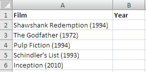
The example below shows a list of five films, each with the year they came out. We want to extract the year from the text and enter it into a different cell. We can then use the year in filters, sorts and PivotTables.

List of films with year of release

The MID function is used to extract a specified number of characters from a text string. However, it needs a starting character. With these films, the starting position varies between each cell. So, MID will need some help.

The FIND function is used to return the starting position of a character. Because the year is enclosed in brackets, the FIND function can be used to find the opening bracket of each cell and it give its position to the MID function as an index number.

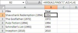
The formula entered in cell B2 is shown below.

=MID(A2,FIND("(",A2)+1,4)

The +1 is used so that the MID function starts from the character after the opening bracket.

MID and FIND functions in Excel extracting text

Excel has many useful text functions. Notably, the LEFT (beginning) and RIGHT (end) functions are also used to extract text from a cell. The FIND function can also be used with those functions to assist with irregular strings.

[Read more…] about Use the MID and FIND Functions to Extract Text

Formula to Match Records on Different Worksheets

I was presented with a problem yesterday where somebody had two sheets of records. They were the same records but one list contained 16000 entries and the other had 14000. The person needed to know what records were missing from the sheet with fewer records.

This required matching records from different worksheets using multiple conditions. To check if they were a duplicate, the first name, last name and company fields needed to match.

To achieve this I wrote an array formula using the IF and SUMPRODUCT functions. This can be seen below testing the data from columns A, B and C across both sheets

{=IF(SUMPRODUCT(((Sheet1!$A$2:$A$16000)=A2)*((Sheet1!$B$2:$B$16000)=B2)*((Sheet1!$C$2:$C$16000)=C2))=1,”Yes”,””)}

An array formula has curly braces at the ends which are added when you press Ctrl + Shift and Enter to run the formula.

The SUMPRODUCT formula returns true if you all three conditions match. THE IF function then displays the word Yes if there is a match on a record, and nothing if there is no match.

The column than then be filtered by blank cells to return all the missing records.
Find out more about the SUMPRODUCT function.

How would you have solved this problem? Drop me a comment with other formulas that could have achieved the same result.

  • « Go to Previous Page
  • Page 1
  • Interim pages omitted …
  • Page 17
  • Page 18
  • Page 19

Primary Sidebar

Recent Posts

  • Excel SWITCH Function – Nested IF Function Alternative
  • Sum Formulas Only in Excel
  • How to Calculate Age in Excel
  • Custom Sort in Excel
  • Case Sensitive Lookup with XLOOKUP in Excel
Advanced Excel Success book

Footer

Contact

[email protected]

LinkedIn Twitter YouTube

Useful Links

  • Home
  • Excel Online Courses
  • Tutorials
  • Sitemap
  • Privacy Policy
  • Jobs by Jooble

Course Topics

  • Blog
  • Charts
  • Courses
  • Dashboards
  • Downloads
  • Excel Tips
  • Formulas
  • Mail Merge
  • Office
  • PivotTables
  • Power BI
  • Power Pivot
  • Power Query
  • VBA

Join Our Mailing List

© Copyright 2009 Computergaga · All Rights Reserved ·