5 SUMPRODUCT Function Examples

In this blog post, we look at 5 SUMPRODUCT function examples. This is one of the great functions of Excel. A function that can turn you from being an Intermediate/Advanced Excel user to an Excel guru instantly.

The SUMPRODUCT function is powerful, versatile and expansive. It is the go to function when looking for an alternative to array formulas.

Ok, are you ready to rock on with these 5 awesome SUMPRODUCT examples?

Let’s do this.

If you prefer to watch videos, check out this video covering the tutorials from this blog post.

Count and Sum the Values for a Specific Month

In the first of our SUMPRODUCT function examples, we will use the SUMPRODUCT function to return the count and sum of the values from a specific month.

In this example the formula below has been entered into cell E3 to count the values for the month specified in cell D3.

=SUMPRODUCT(--(MONTH($A$2:$A$12)=$D$3))

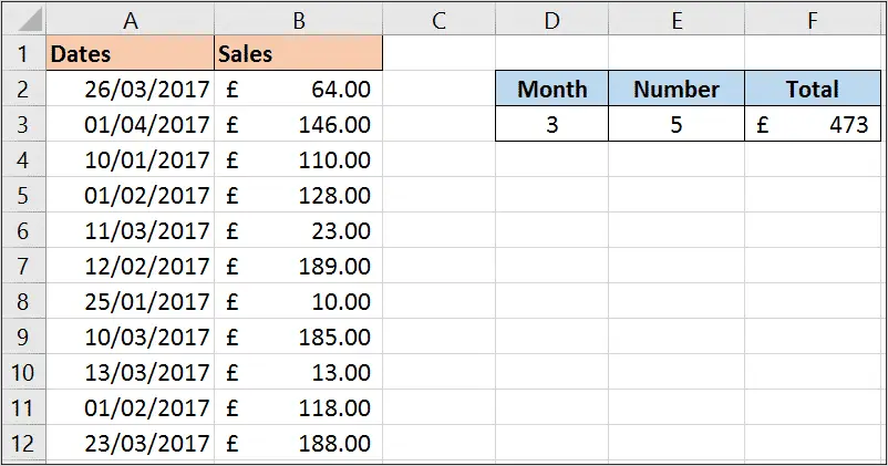
SUMPRODUCT example to sum or count values for a specific month

The MONTH function has been used to extract the month from the each date in the range. This is then tested to see if it is equal to the month we want to count.

The double hyphens ‘–‘ are used to convert the true and false responses of this logical test to 1 and 0. The SUMPRODUCT then sums these 1’s and 0’s to return the answer.

The formula below has then be entered into cell F3 to return the total sales value for that month.

=SUMPRODUCT(--(MONTH($A$2:$A$12)=$D$3),B2:B12)

For this we just needed to add a comma and then the range of cells containing the sales values.

This works because the SUMPRODUCT function multiplies the 1’s and 0’s from month test by these sales values. And then these results are all summed.

Count the Occurrences of Specific Words from a Range of Cells

This example can be very useful if you have to analyse comments, feedback or SEO keyword data. In these situations you will have large volumes of text and you may be looking for the occurrence of specific words.

In this example, the SUMPRODUCT formula has been used in cell D2 to count all the occurrences of words entered in cell C2.

=SUMPRODUCT(--(ISNUMBER(FIND(C2,A2:A9))))

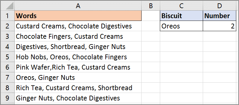
Count instances of words in a range with this SUMPRODUCT function example

In this formula, the FIND function searches for the words in each cell. If the words are found then FIND returns its starting position, and if not it returns and error value.

The ISNUMBER function will then return true if a number is returned, or false if not. The double hyphens are then used just like the previous example to convert the true and false to 1 and 0.

The 1’s and 0’s are then summed by SUMPRODUCT to return the final count.

Count Unique Values

The SUMPRODUCT function can also be used to perform a unique count of values in a range.

Being able to count how many orders and how many training sessions is great. But sometimes you need to know how many different customers placed orders, and how many different training sessions. Then you need a unique count.

The formula below performs a unique count on range A2:A10.

=SUMPRODUCT(1/COUNTIF(A2:A10,A2:A10))

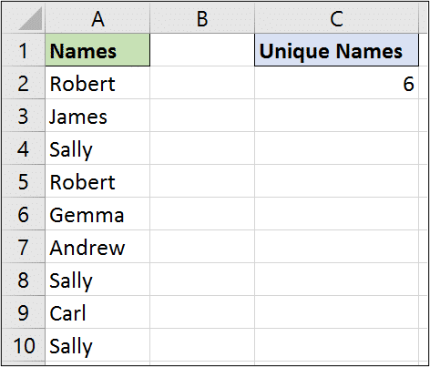
Count the unique values only with SUMPRODUCT and COUNTIF

For this to work, the COUNTIF function counts the occurrences for each name in the list producing the below. This says that Robert occurs twice, James once and Sally three times etc.

=SUMPRODUCT(1/{2;1;3;2;1;1;3;1;3})

These values are then divided by the 1 producing the below.

=SUMPRODUCT({0.5;1;0.33;0.5;1;1;0.33;1;0.33})

And then SUMPRODUCT sums them all up delivering the unique count.

Sum the Top 3 Values from a Range

How about summing only the top values from a range. Yes SUMPRODUCT can do this.

In this example, we sum only the top 3 values, but this can easily be adapted to top 5, top 10 or whatever you wish.

The formula below sums only the top 3 values in range B2:B12.

=SUMPRODUCT(LARGE(B2:B12,{1,2,3}))

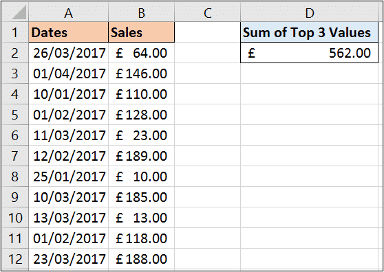
SUMPRODUCT function example to sum the top 3 values in a range

This formula uses the LARGE function with SUMPRODUCT. The LARGE function is used to return kth largest value in a data set, such as the 5th largest.

In this example we have provided the LARGE function with an array of {1, 2, 3} so that it returns the top 3. The SUMPRODUCT then sums them.

This is all in the beauty of the SUMPRODUCT formula handling arrays of data.

If you need to sum the values from the bottom of the range you can use the SMALL function.

Perform a Two Way Lookup with SUMPRODUCT

In the final one of our SUMPRODUCT function examples, we see the SUMPRODUCT formula performing a two way lookup.

You may have created two way lookups before in the past. The most common way to do this is to use the INDEX and MATCH function combination.

The formula below performs a two way lookup. It looks for the value of cell B1 down column A, and the value in cell D1 along row 3. It returns the value at the intersection, which in the image is £246.

=SUMPRODUCT((A4:A13=B1)*(A3:M3=D1),A4:M13)

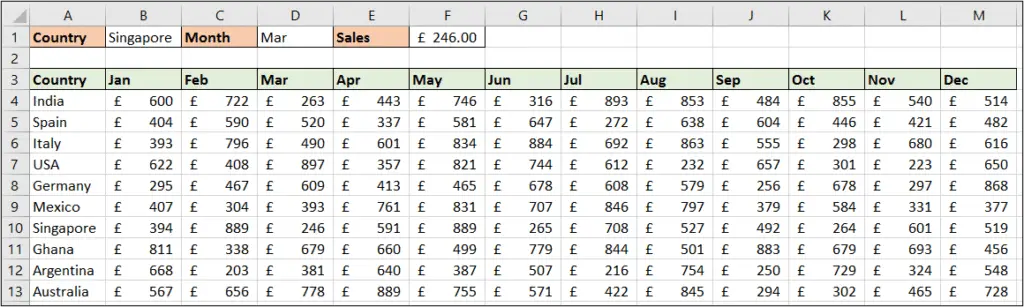
The asterisk (*) is used as an AND operator in this formula. And the second array is the range to return the value from i.e. A4:M13.

This formula is so incredibly versatile we could be listing far more SUMPRODUCT function examples in this tutorial. For example, it can also sum the values from every nth row of a list.

What have you used it for?