The CHOOSE function in Excel chooses a value, range or an action from a list of values, ranges and actions, dependent upon a given index number.
The Excel CHOOSE function is a simple, yet very effective Excel function. There are many brilliant examples of its use, and we will explore some of them in this tutorial.
Download the Excel workbook used in the tutorial to practise.
Excel CHOOSE Function Syntax
The CHOOSE function has a very straight forward syntax. It requires the index number and the list of possible values, ranges and actions.
=CHOOSE(index_num, value1, [value2], ...)
- Index num: The index position in the list from which to return the value, range or action.
- Value1, value2, …: The list of values, ranges or formulas that you want CHOOSE to return.
Return the Fiscal Quarter with the CHOOSE Function
In the first CHOOSE function example, we will return the fiscal quarter from a given date.
For this example, the fiscal year begins on the 1st April. So, the list below describes the quarter and which month belongs to it.
- Q1 = Apr, May, Jun
- Q2 = Jul, Aug, Sep
- Q3 = Oct, Nov, Dec
- Q4 = Jan, Feb, Mar
This calculation lends itself nicely to the CHOOSE function. We can provide CHOOSE with a list of the quarter numbers, and match the month numbers against the indexes of that list.
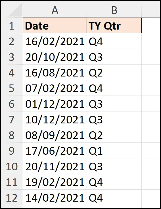
The following formula returns the fiscal quarter for the dates in column A.
="Q"&CHOOSE(MONTH(A2),4,4,4,1,1,1,2,2,2,3,3,3)
The MONTH function is used to extract the month number from the date for use. The Excel CHOOSE function result is appended to the “Q” using an ampersand ‘&’.
Dynamic SUM Function
In this second example, we will use the CHOOSE function to return a range to be summed by the SUM function. This range will be specified from a drop-down list value.
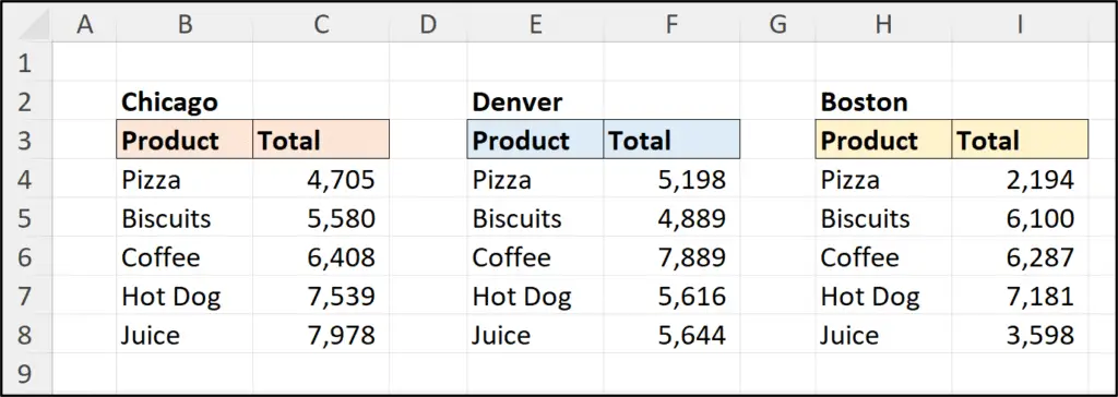
The following image, shows three different ranges of product sales data. Each range relates to a different city – Chicago, Denver and Boston.
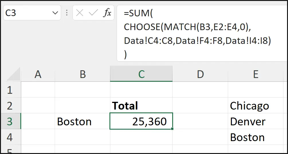
In the following formula, the MATCH function is used to return an index number for the position of the city in cell B3, in the range E2:E4. It is important that the order of the cities in range E2:E4, match the list of ranges order in the CHOOSE function.
=SUM(
CHOOSE(MATCH(B3,E2:E4,0),
Data!C4:C8,Data!F4:F8,Data!I4:I8)
)
This formula is split over multiple lines to make it more readable. This is done by pressing Alt + Enter in the Formula Bar.
The Excel CHOOSE function returns the range for the selected city to be summed.
Return a Range with the CHOOSE Function in Excel
Instead of returning a range to a function such as SUM, the range could be returned to the sheet. This dynamic range could then be used as the source for a chart, drop-down list or other Excel feature.
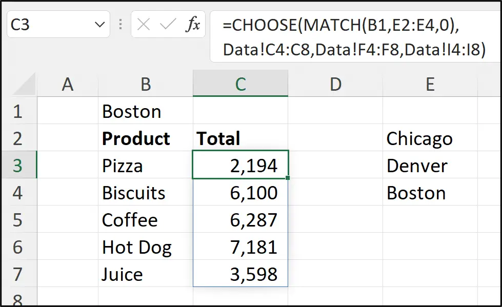
The following formula is similar to the previous one. This time there is no SUM function and the sheet layout is slightly different. The drop-down list is in cell B1.
This version of the formula works only for those with a dynamic array powered version of Excel.
=CHOOSE(MATCH(B1,E2:E4,0),
Data!C4:C8,Data!F4:F8,Data!I4:I8)
Use the following formula, and fill the formula down to cell C7 if you’re using an older version of Excel.
=CHOOSE(MATCH($B$1,$E$2:$E$4,0),
Data!C4,Data!F4,Data!I4)
CHOOSE a Formula to perform
For a final example, we will return a formula with the CHOOSE function in Excel.
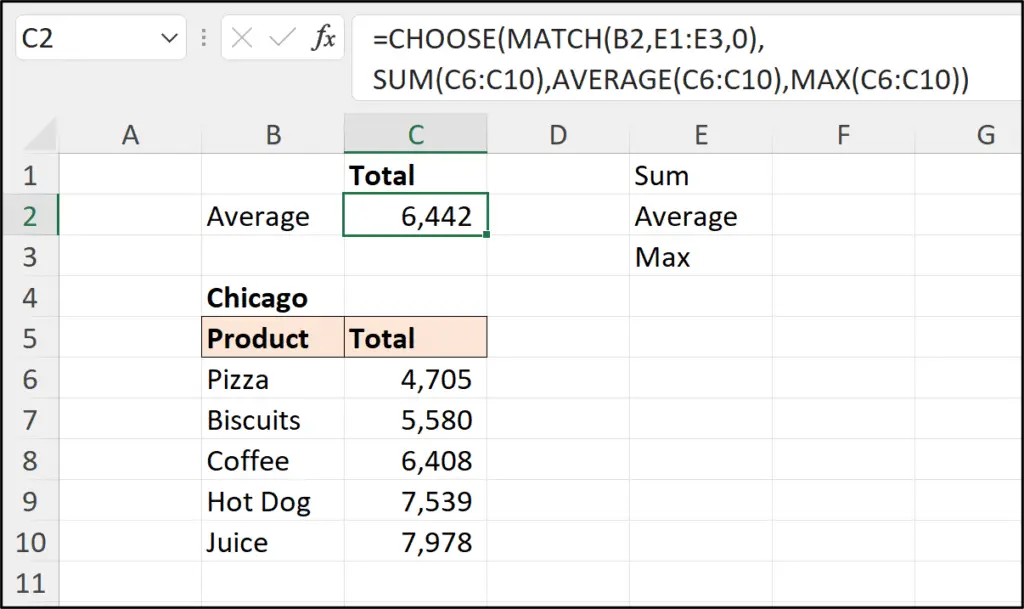
The following formula uses a similar setup to the two previous examples. The MATCH function now returns the index of the selected calculation from range E1:E3. The Excel CHOOSE function then performs the selected calculation from its list.
=CHOOSE(MATCH(B2,E1:E3,0),
SUM(C6:C10),AVERAGE(C6:C10),MAX(C6:C10))
The CHOOSE function in Excel has a very simple structure, but simple is good. Hopefully, the examples in this tutorial have shown you useful this function can be.
It’s ability to return values, ranges or formula from its list makes it incredibly versatile. It is also available to all versions of Excel, so is reliable when collaborating externally to your organisation.


