The GETPIVOTDATA Function in Excel

The GETPIVOTDATA function in Excel is used to query and extract data from a PivotTable. It is essentially a PivotTable lookup formula.

This function can be extremely useful. When your PivotTable updates, it may grow or reduce in size, or the field items may change order – GETPIVOTDATA will continue to extract the correct data.

In this blog post, we will show why the GETPIVOTDATA function in Excel is useful with an example, but then show an example of when we do not want it, and how we can turn the feature off.

Watch the Video

Using the GETPIVOTDATA Function in Excel

The function is switched on by default so when you write a reference to the cell of a PivotTable, the GETPIVOTDATA function is used.

For example, if I click in a cell and type =, and then click on cell D9 of the PivotTable below, the following function is entered.

=GETPIVOTDATA("Total Sales Value",$A$3,"Product Category","Grains/Cereals","Years",2012)

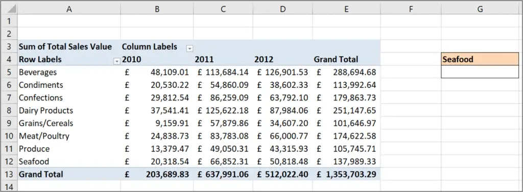
This says to extract data from the Total Sales Value field of the PivotTable found in cell A3. Cell A3 is the top left corner cell of the PivotTable. It could have been any cell, but the top left corner is always chosen by default.

It then specifies to retrieve the value from the Grains/Cereals item of the Product Category field, and the 2012 item of the Years field.

So it is a very specific and structured reference. If the PivotTable changes in layout, it continues to retrieve the right data. While I cannot be sure that cell D9 would have been the value I wanted.

Making the GETPIVOTDATA Function Dynamic

For those that do not like the GETPIVOTDATA function in Excel (and there are many), the argument will be that it is too structured.
So in this example, lets make it more dynamic.

Using the same PivotTable as before, I have inserted a drop down list in cell G4. This is a list of the different product categories.

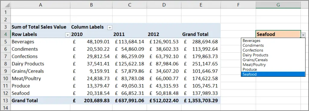
So instead of having a GETPIVOTDATA function returning data like this.

=GETPIVOTDATA("Total Sales Value",$A$3,"Product Category","Seafood")

I could reference cell G4, so that whatever category I select the correct value is returned.

=GETPIVOTDATA("Total Sales Value",$A$3,"Product Category",G4)

Combining this useful function with cells on a spreadsheet that contain formulas, or form controls, gets the most out of it.

And for those that dislike the GETPIVOTDATA function due its structured nature, it takes that argument away.

When GETPIVOTDATA Does Not Help

In this example, I have a PivotTable with a Country filter and the Product Category values sorted in a descending order so that the largest values are at the top.

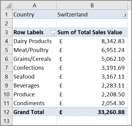
Now if somebody uses the filter to change the country, the PivotTable values will move.

So lets imagine I want to return the value of the best selling product category from the PivotTable.

If I type = into a cell and then click on cell B4 (the cell containing the value of the best selling product category), the following GETPIVOTDATA function would be written.

=GETPIVOTDATA("Total Sales Value",$A$3,"Product Category","Dairy Products")

But I am not interested in dairy products. That just happens to be the best seller in this country. If I change the country, it could be a different product category in the number 1 position.

So instead I would just type =B4. By typing in the reference, it bypasses the GETPIVOTDATA function.

Turning Off GETPIVOTDATA

If you do decide that the function is not helping you much in how you want to reference PivotTable data. You can switch it off.

Then when you click on the cells of a PivotTable, Excel will use normal spreadsheet references instead of GETPIVOTDATA.

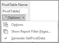
To do this;

1. Click on the PivotTable and click the PivotTable Analyze tab on the Ribbon.
2. Click on the list arrow for the Options button on the far left side and click Generate GetPivotData.

More PivotTable Tutorials

• Ranking fields in a PivotTable
• 5 advanced PivotTable tutorials
• Count unique values in a PivotTable
• 4 ways to group times in Excel