• Skip to main content
  • Skip to primary sidebar
  • Skip to footer

Microsoft Excel Tips and Tricks - Computergaga

  • Home
  • Excel Online Courses
  • Excel Functions List
  • Free Downloads
  • Blog
  • Tutorials
  • About
Home / PivotTables / Rank Fields in a PivotTable in Excel

Rank Fields in a PivotTable in Excel

In Excel, one of the PivotTable calculation options is to rank fields in a PivotTable.

Yes, you can sort the fields of a PivotTable to view items in order from largest to smallest, or smallest to largest depending on what you are trying to achieve. But you may wish to keep your list of products, customers, salespersons or whatever the field is your are ranking in alphabetical order.

Take the table below for instance. This PivotTable displays the number of sales and conversion rate for the members of a sales team.

PivotTable with sales and conversion rate

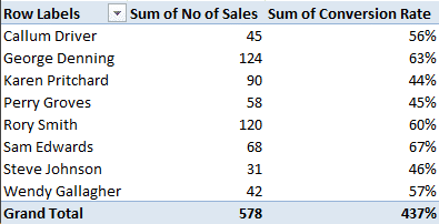
We would like to add a rank field to the PivotTable for both fields.

Add a Rank Field in a PivotTable in Excel

  1. Add the field to the PivotTable that you want to use for ranking. In this case the No of Sales and Conversion Rate fields would be added again.
  2. Right mouse click on a value in the field you want to rank and select Show Value As > Rank Largest to Smallest.
Rank PivotTable fields largest to smallest
  1. The ranking field is introduced. Repeat for any other fields of the table.
  2. Rename the column headings so that they no longer say Sum of **.
PivotTable with two rank fields

At this point the fields showing the value can be removed. The rank field can stand on its own and the other field is not necessary.

Watch the Video

Related Posts:

  • What You Need to Know About Dynamic Array Formulas in Excel
    What You Need to Know About Dynamic Array Formulas in Excel
  • Create a Picture Lookup in Excel
    Create a Picture Lookup in Excel
  • Entering Fractions in Excel
    Entering Fractions in Excel
  • Advanced Excel Skills
    Advanced Excel Skills

Reader Interactions

Comments

  1. Gulfaz says

    20 September 2017 at 5:02 am

    Not Needed,
    Please Explain the Use of Get Pivot

    Reply

Leave a Reply Cancel reply

Your email address will not be published. Required fields are marked *

Primary Sidebar

Popular Posts

  • Excel Fixtures and League Table Generator
  • 5 Reasons Why your Excel Formula is Not Calculating
  • Excel IF Function Contains Text – A Partial Match in a Cell
  • Excel Formula to Display the Sheet Name in a Cell
  • 4 Alternatives to Nested IF Formulas
  • How to Hyperlink to a Hidden Worksheet in Excel
  • How to Create a Reverse FIND Formula
  • Check if a Value is an Even Number
  • IF Function in Power Query Including Nested IFS
  • Conditional Formatting Multiple Columns – 3 Examples

Recent Posts

  • SEQUENCE Function in Excel
  • Sort by Drop Down List in Excel
  • Advanced SUM Function Examples – The Power of SUM
  • Display Negative Time in Excel
  • Lookup Multiple Values in Excel
Advanced Excel Success book

Footer

Contact

[email protected]

Useful Links

  • Home
  • Excel Online Courses
  • Tutorials
  • Sitemap
  • Privacy Policy
  • Jobs by Jooble

Course Topics

  • Charts
  • Courses
  • Dashboards
  • Downloads
  • Excel Tips
  • Formulas
  • Mail Merge
  • Office
  • PivotTables
  • Power BI
  • Power Pivot
  • Power Query
  • VBA

Join Our Mailing List

© Copyright 2020 Computergaga · All Rights Reserved ·