Sum Formulas Only in Excel

A unique use case for summing values, could be to sum formulas only in Excel.

The SUM function will sum all numeric values in a given range, but you may have a range interspersed with other formulas that calculate subtotals or perform conditional calculations.

So, how do you only sum the cells that contain formulas. Let’s find out.

Watch the Video – Sum Formulas Only

The Sample Data

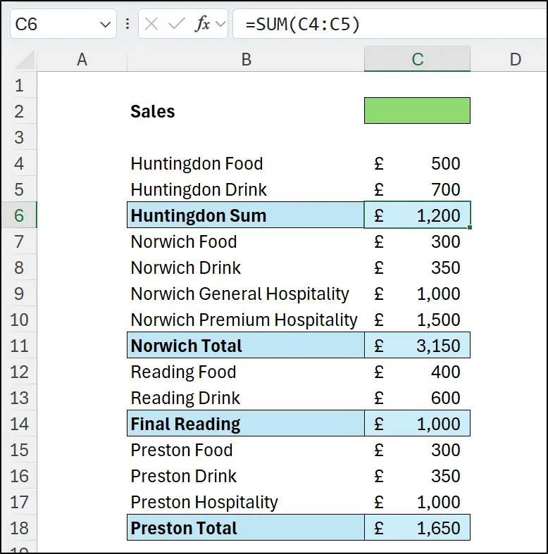
For this example, we have the following data. In column C, we have a range of values that includes formulas that use a SUM function (this could be any formula).

These formula cells are in irregular spaced rows so we cannot use our sum every Nth row technique. They also have irregular labels such as “Huntingdon Sum” and “Norwich Total”, so we cannot deploy a SUMIFS formula. The only thing that identifies these values is that they contain a formula.

Using the ISFORMULA Function

Using column D, we will build a formula to first identify these values, and then sum them. We will use column D to understand how this works.

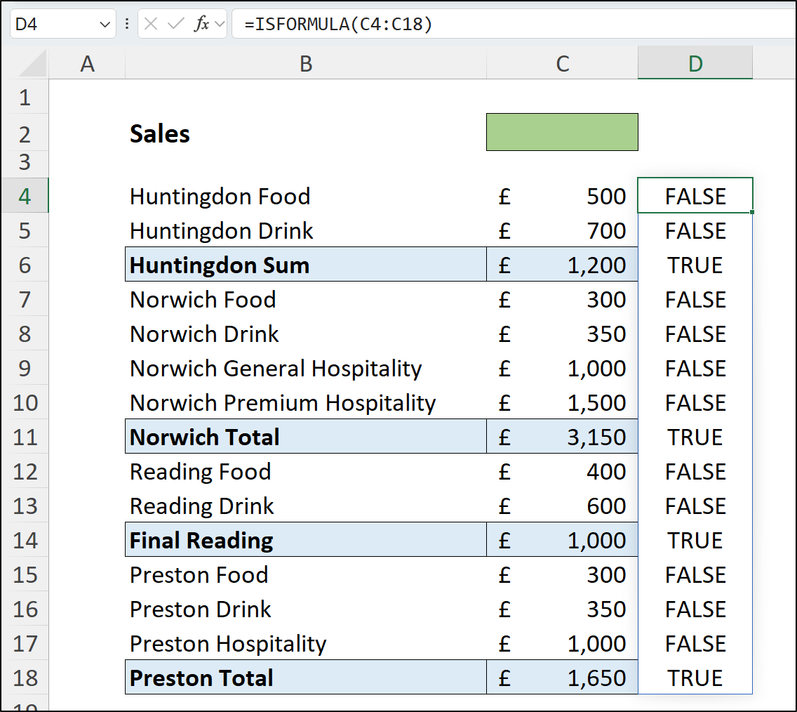
Firstly, we will use the ISFORMULA function. This function returns TRUE if a cell contains a formula, otherwise FALSE is returned.

This can be seen in the results of this formula.

=ISFORMULA(C4:C18)

Converting TRUE and FALSE to 1 and 0

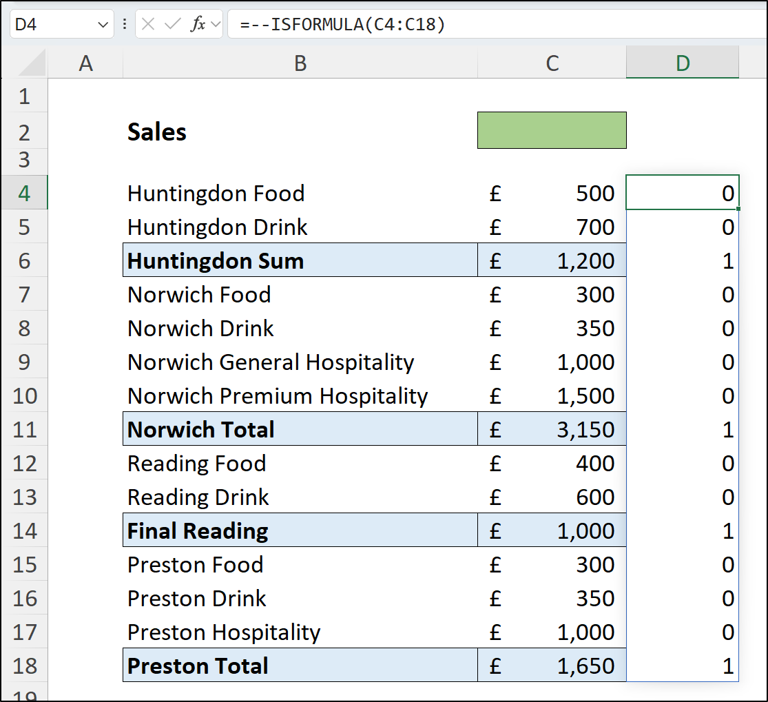
Our goal is to use the results of the ISFORMULA function in an operation with the values to be summed. So, we need to convert the TRUE and FALSE values to the numeric values of a 1 and 0.

My preferred way of doing this is to use the double unary (two negative operators) before the formula as shown below.

Other methods would include using the N function of Excel or using a mathematical operation that does not affect the result such as +0 or *1.

SUMPRODUCT to Finish

Finally, we want to calculate the product of the corresponding values in columns C and D, and then sum those products.

Excel has the ideal function for this task – the SUMPRODUCT function.

We will finish by copying the formula we have in column D and using it a SUMPRODUCT formula in cell C2.

=SUMPRODUCT(–ISFORMULA(C4:C18),C4:C18)

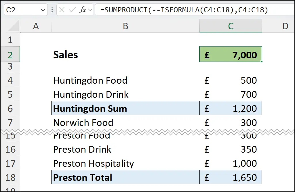
This formula multiplies the corresponding values from the result of the ISFORMULA formula and those in range C4:C18. The results of this multiplication, or product, is then summed.

For example, it performs 0*500, 0*700, 1*1200, 0*300 and so on. And then sums these results without the need for a helper column.

In modern versions of Excel, the SUM function can be used instead of SUMPRODUCT. This is demonstrated in my article on advanced SUM function examples.

However, SUMPRODUCT was born for this task, so would be rude to not use it ?

A Possible Alternative

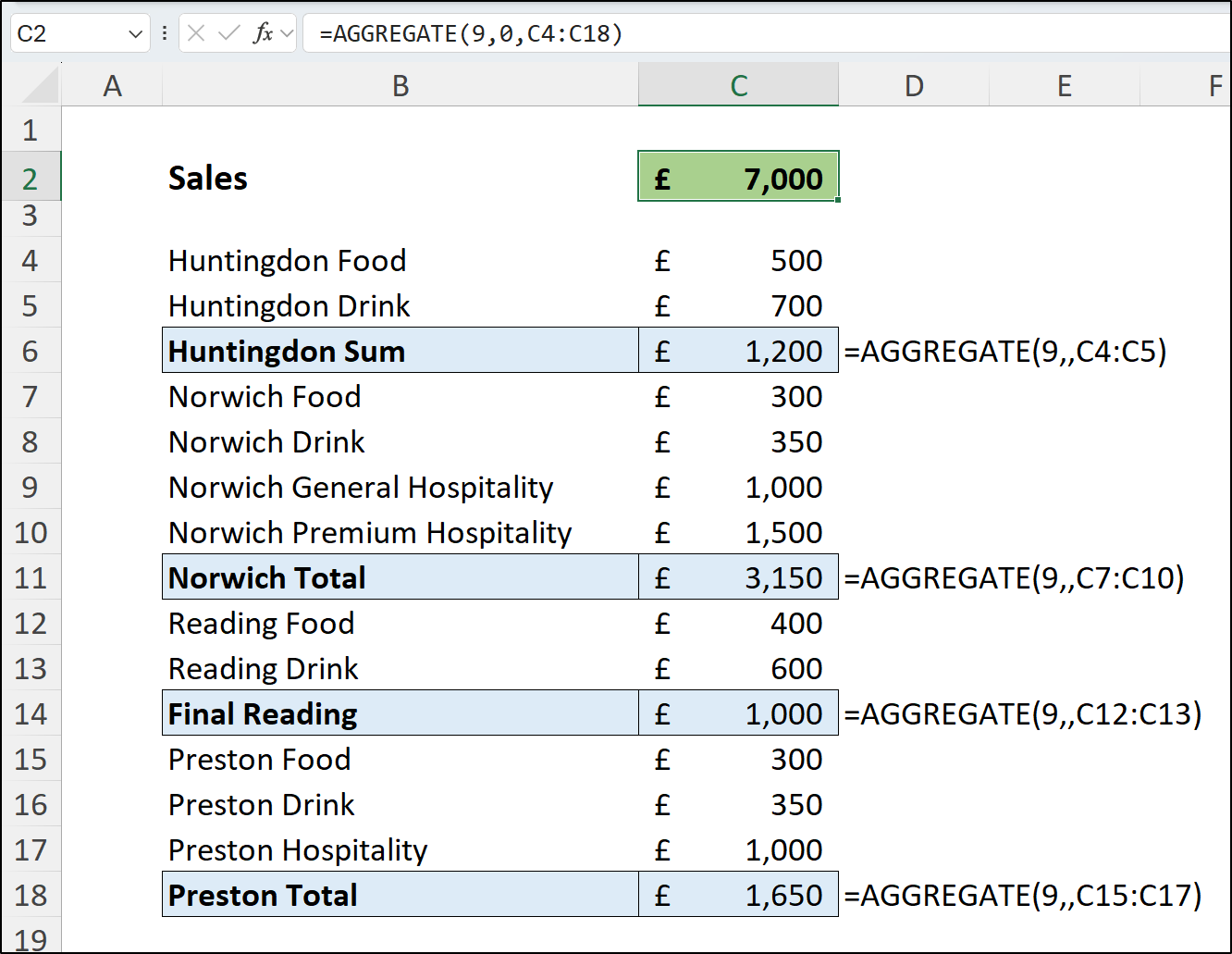
In this specific example, an alternative approach could be to use the SUBTOTAL or AGGREGATE function instead of the Excel SUM function for the subtotals. You could then use one of these functions again, AGGREGATE is better, to sum all values except the subtotals.

In the following example, column D shows the formula used for the subtotals instead of SUM. The formula in cell C2 is shown in the formula bar. The 9 in the AGGREGATE function specifies the sum operation (it can perform many other functions), and the 0 states to ignore subtotals in the range.

This is an awesome approach, however it only works when ignoring subtotals in a range, while the technique to sum formulas only would work for any formula, including text operations and conditional functions such as IF, making it more versatile.