• Skip to main content
  • Skip to primary sidebar
  • Skip to footer

Microsoft Excel Tips and Tricks - Computergaga

  • Home
  • Excel Online Courses
  • Excel Functions List
  • Free Downloads
  • Blog
  • Tutorials
  • About
Home / Formulas / Sum a Column Ignoring Formula Errors

Sum a Column Ignoring Formula Errors

Having formula errors on a spreadsheet can be bad news. They look ugly, they frighten the less Excel experienced among us and they stop our other formulas from working.

If you have formula errors on a spreadsheet it is normally best to stop it at its source. To either correct the error, or to hide it using formulas such as ISERROR and IFERROR.

However, if your spreadsheet is large, having these IFERROR functions in every cell to protect against error values will add more calculation time to your spreadsheet.

There is a function in Excel called AGGREGATE which allows us to perform various functions on a range whilst ignoring formula errors.

Using AGGREGATE to Ignore Error Values

The worksheet below contains formula errors that we want to ignore when calculating the total investment.

Table of data including errors

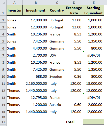
The following formula can be written into cell E17.

AGGREGATE function to sum values and ignore errors

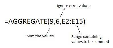
There is a lot more to the AGGREGATE function. For example, it can also be used to ignore hidden rows and subtotals. And it can perform 19 different functions in all so is not limited to only summing values.

Watch the video below to see the AGGREGATE function being used to sum values whilst ignoring error messages.

Related Posts:

  • How to Make Table Column References Absolute
    How to Make Table Column References Absolute
  • Excel Formula to Find the Cell Address of a Value
    Excel Formula to Find the Cell Address of a Value
  • Advanced SUM Function Examples - The Power of SUM
    Advanced SUM Function Examples - The Power of SUM
  • Multiple Condition Lookup Formula in Excel
    Multiple Condition Lookup Formula in Excel

Reader Interactions

Comments

  1. sorin says

    14 August 2015 at 8:14 am

    Thank you very much.
    I want to receive updates always.

    Reply
  2. Gita says

    11 October 2017 at 9:07 am

    Thank you!!

    Reply
  3. Nida says

    18 March 2021 at 7:24 am

    This is my new “all time favourite” formula!!! Thanks a stack!

    Reply
    • Alan Murray says

      19 March 2021 at 11:44 am

      Excellent! My pleasure.

      Reply

Leave a Reply Cancel reply

Your email address will not be published. Required fields are marked *

Primary Sidebar

Recent Posts

  • LIVE Currency Exchange Rate in Excel
  • N Function in Excel
  • Non-Adjacent Columns with FILTER Function
  • Moving Average in Excel
  • Excel IMAGE Function – Insert Images from a Cell Value
Advanced Excel Success book

Footer

Contact

[email protected]

Useful Links

  • Home
  • Excel Online Courses
  • Tutorials
  • Sitemap
  • Privacy Policy
  • Jobs by Jooble

Course Topics

  • Charts
  • Courses
  • Dashboards
  • Downloads
  • Excel Tips
  • Formulas
  • Mail Merge
  • Office
  • PivotTables
  • Power BI
  • Power Pivot
  • Power Query
  • VBA

Join Our Mailing List

© Copyright 2009 Computergaga · All Rights Reserved ·