Sort by Drop Down List in Excel

In this tutorial, we see how to sort by drop down list in Excel.

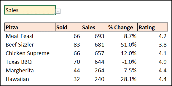
We have a table containing details about pizza and their performance such as the feedback rating, how many have been sold and the % change from the previous pizza data.

We want to be able to select the column to sort by from a drop down list, and then the table will be automatically sorted by the chosen column.

Watch the video, or read on for the full tutorial.

The tutorial uses the power of the array engine of Excel to sort by drop down list. However, there is another video at the end of the tutorial that shows how to do this in all versions of Excel.

Download the sample workbook to follow along.

The Data

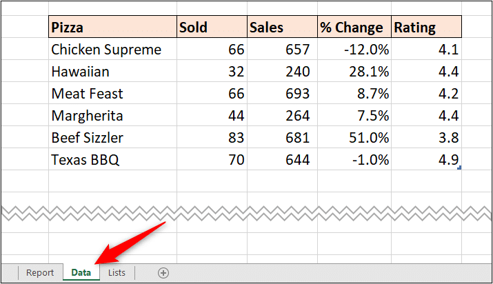
On the sample workbook provided, there is a Data tab that contains the pizza data that we want to sort. This data is formatted as a table named tblPizza.

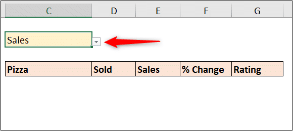
On a separate worksheet named Report, We have a drop down list in cell C2 containing all the column headers from the tblPizza table already created.

The headers are enter in range C4:G4 ready. We need to write the required formulas to return the data from the tblPizza table, and sort them by the value selected from the drop down list.

Return the Selected Header

The first task is to return the header selected from the drop down list. We need to know which header was selected before we can sort by that column.

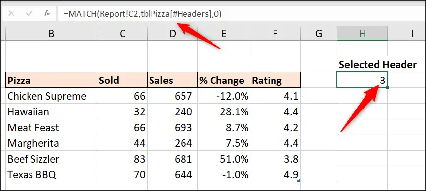
The following MATCH function was entered into cell H3 of the Data sheet to achieve this.

=MATCH(Report!C2,tblPizza[#Headers],0)

This function looks for the value selected from the drop down, along the header row of the tblPizza table, and returns the index number of that column. For example, Pizza is column 1, Sold is column 2 and so on.

Formula to Sort By Drop Down Value

We can now write a formula to return all columns from tblPizza and sort them by the selected drop down value. For this, we will use the SORT function in Excel.

The following SORT function is entered into cell C5 of the Report sheet.

=sort(tblPizza,Data!H3,if(Data!H3=1,1,-1))

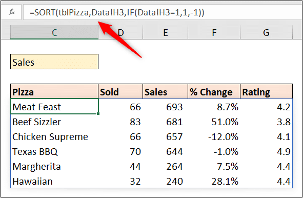
This formula sort all columns of tblPizza by the value in cell H3 of the Data sheet. This is the column selected from the drop down list.

The IF function is used to apply a different sort order dependent upon the chosen column.

If column 1 is chosen, this is the pizza names, so sort them in ascending order. Number 1 is entered to specify ascending order to the SORT function.

Otherwise, if any other column is selected, -1 is entered to specify the descending order.

And that is it!

Very easy to do in modern Excel with the array formula engine and the SORT function.

Sort By Drop Down Value – All Versions

So, how would this be done in older versions of Excel that do not contain the array engine or the SORT function?

I will show you my approach in the following video.

Download the sort by drop down in all versions workbook to follow along with the video.

The approach uses some of the best functions of Excel that are compatible with all Excel versions. These include OFFSET, MATCH, INDEX and COUNTIFS.

Many other techniques are demonstrated including how to make table column references absolute and entering formulas into defined names for easier referencing.

I wanted to create a solution that avoided any kind of array formula and used classic drag the fill handle formulas.