Power Query Custom Data Types

This tutorial will take you through the new Power Query custom data types in Excel.

What does this all mean?

Well, you can now create your own data types in Power Query similar to the ones you see on the Data tab (Stocks, Geography, etc).

These rich data types allow us to store many columns of data in just one column. This frees up space on the worksheet.

All columns of data are easily accessible using formulas or by simply typing the column name.

In this tutorial, you will see how to create Power Query data types and how to access their data with formulas.

Download the Files

The example we are using here is an Excel dashboard that I created recently as part of a contest named Excel Hash. This was a contest between myself and 17 other Excel experts.

You can download both files below to follow along with the tutorial.

Download the Excel dashboard

Download the participants workbook

Watch the Video

Get the Data

First, we need to get the data we want to use. For this example, it is coming from an external Excel workbook named participants.

The scenario is that we have 12 members of staff who ran and walked as many miles as possible to raise money for charity. The staff are grouped into teams and have a chosen charity. All of the data is on this participants workbook.

The dashboard ranks the staff by the miles they achieved and performs other calculations.

1. Click Data > Get Data > From File > From Workbook.
2. Locate the participants workbook, select it and click Import.
3. In the Navigator window, select the competitors table and click Transform Data.

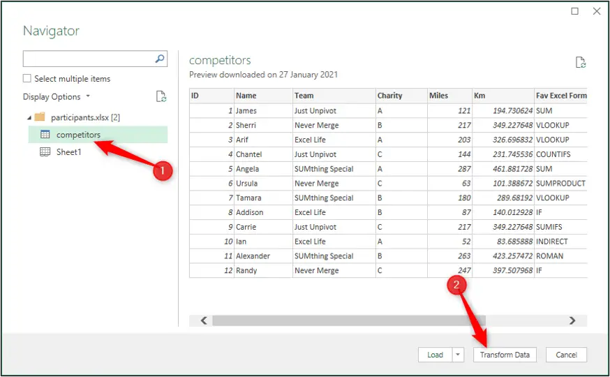
The Power Query Editor opens and shows a preview of the competitors table. We will not perform any transformations in this tutorial, except to create the data type.

Create a Power Query Data Type

You can include any columns you want in the data type. We will use all the columns.

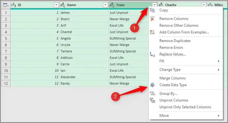
1. Click the ID column header, press and hold the Shift key and click the Pizza or Burger column header to select all the columns.
2. Right click a column and click Create Data type, or click Transform > Create Data Type.

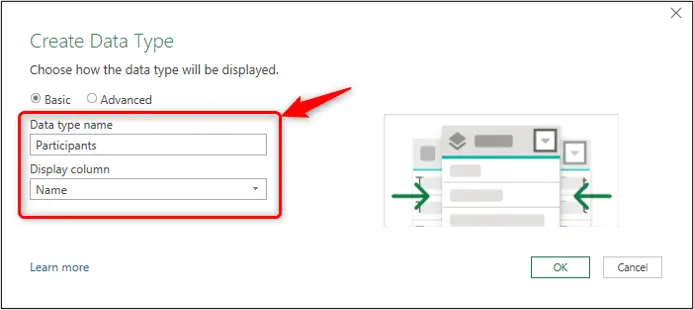
3. In the Create Data Type window, type “Participants” for the Data type name and select Name from the list for the Display column. Click Ok.

All the columns are combined into one record. You can see the custom data type icon in the column header.

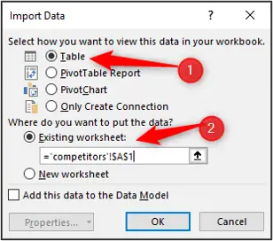
4. Click Home > Close & Load > Close & Load To.
5. Select Table, Existing worksheet and load it to cell A1 of the competitors sheet.

The custom data type is loaded to the worksheet. It is only one column wide so preserves space, yet is rich with data.

View the Data Type Columns

There are a few different ways to easily access the columns of a Power Query data type.

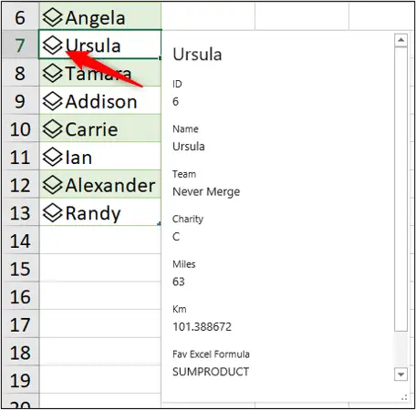
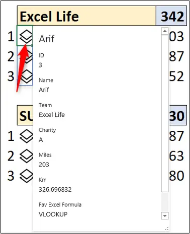
One simple way, is to click on the custom data type icon next to the names of the participants.

A pop up window shows the hidden columns. This includes the number of miles ran, the chosen charity and their favourite Excel formula.

Another option is to display some of the columns physically on the worksheet.

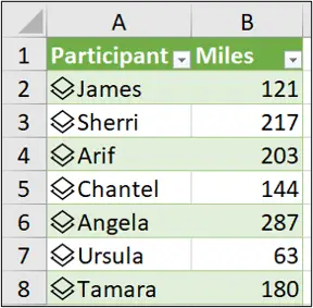
Click the Add Column button next to the table header and click the column you want to add.

In this example, the Miles column has been added to the worksheet.

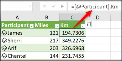
You can also add a column by typing the column name into the header row of the table.

In this example, the kilometres run is being added by typing the column header Km into an empty cell on the header row.

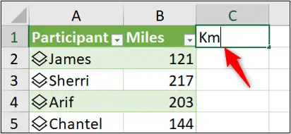
The typed header is matched to a custom data type header. Amazing!

You can also see the formula that was used to fetch this data.

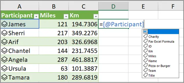
So, a final method would be to write a formula to add a column.

Type “=”, click the participant name and a list appears with the columns to choose from. Very easy.

Formulas and Power Query Custom Data Types

Now, you do not need to add a column to the worksheet in order to use the columns from the data type. We can access them directly with formulas.

Let’s look at three examples of popular Excel formulas using the custom data type data.

We will start with a simple SUM function.

The following formula has been used in cell J2 of the dashboard to sum the total miles ran by all participants.

=SUM(competitors[Participants].Miles)

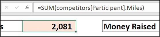
• Competitors – the name of the table
• Participant – the name of the data type column
• Miles – the name of the column within the data type that we want to use

Let’s take that a step further and use an XLOOKUP function to get data from the Power Query custom data type.

The following formula has been used in cell J4 to return the team that the winner (Angela in cell AH2) belonged to.

=XLOOKUP(AH2,competitors[Participant].Name,competitors[Participant].Team)

Finally, we will see an example of the FILTER function being used with the data type.

This example, is especially interesting because we will return the entire data type, not a single column of data.

The formula below has been used in cell E9 of the dashboard.

=SORTBY(
FILTER(competitors,competitors[Participant].Team=E8),
FILTER(competitors[Participant].Miles,competitors[Participant].Team=E8),
-1)

The array of the FILTER function is competitors. This returns the entire table and not just a specific column.

The SORTBY function is also used to order the data types by the number of miles ran.

You can see the data type icon next to the returned names in the image below. There is also the add column button to quickly insert additional columns if we wanted.

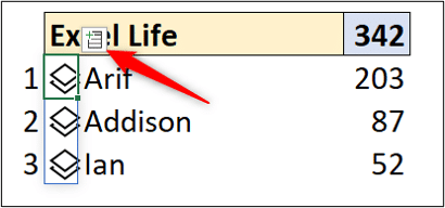
By returning the entire custom data type, we can quickly view extra information on our dashboard by clicking the data type icon.

So, I hope this tutorial provided a nice over view of the Power Query custom data types and what they can offer.

I’m sure there are more exciting things to come in this space.