In this tutorial, we will use Excel formulas to lookup multiple values and combine the results into a single cell, or row. We will also order the returned values in two different ways.
The formulas used in this tutorial are only available in Excel 365 and Excel Online. They take advantage of the array engine of modern Excel. This video show you how to lookup multiple values in all Excel versions.
Watch the video below, or read on. This tutorial covers three examples of a lookup formula to return multiple values.
Lots of information, so let’s dive into the action.
Download the workbook to follow along with the tutorial.
Lookup and Return Multiple Values as a List
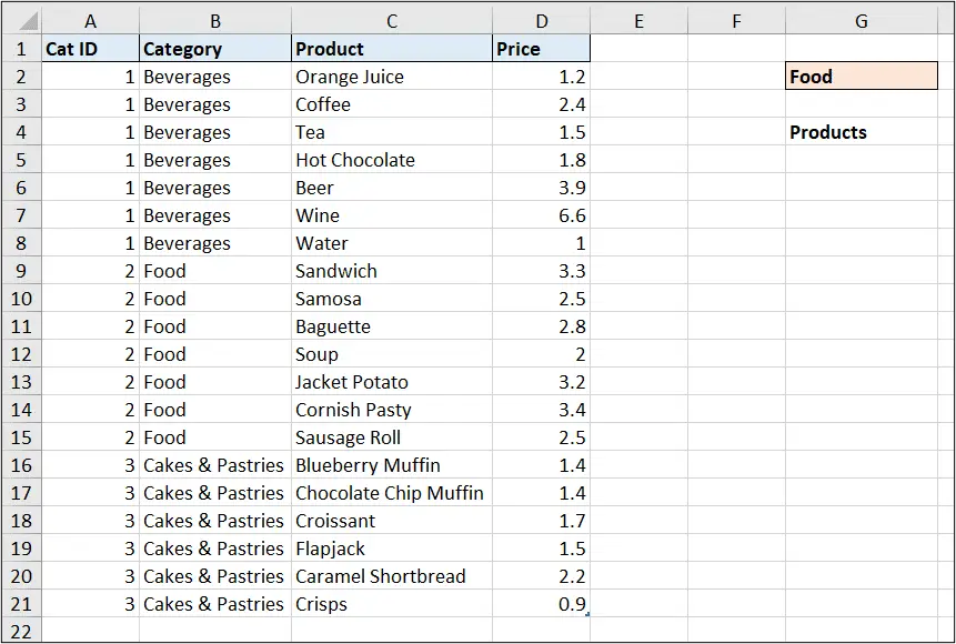
In this example, we have a table named ‘products’ which contains a product name and the category it is assigned to. In cell G2, there is a drop-down list that can be used to select one of the three product categories – Beverages, Food or Cakes & Pastries.
We want to return all the products from the specified category into the range under ‘Products’ beginning in cell G5.
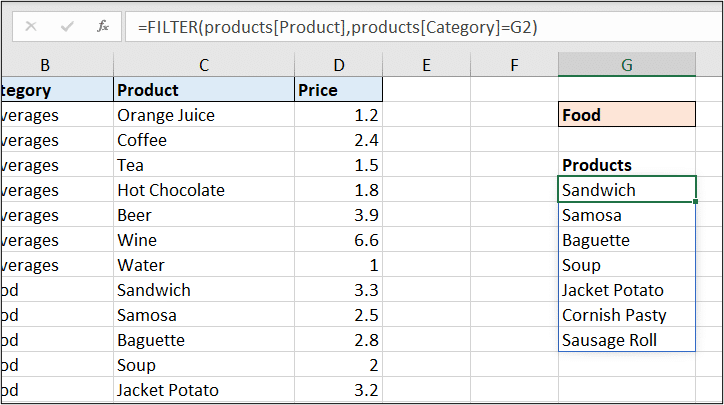
In cell G5, the following formula is used.
=FILTER(products[Product],products[Category]=G2)
The FILTER function in Excel is a lookup formula that returns multiple values, so this task is tailor made for it.
The first argument is the values to return. In this example, that is the ‘Product’ column. The second argument is the criteria, which is if the category is equal to that selected in cell G2.
This formula easily returns multiple values. The formula is entered into cell G2 only, and spills the results to the adjacent cells.
Combine the Values into One Cell
Let’s now take this a step further and combine the results into a single cell. We will also order the product names alphabetically.
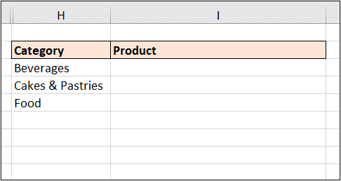
Continuing with the ‘products’ table, we now have the following range and would like to return the results of all products for each of the categories. These results will be combined into a single cell and separated by a comma.
The following formula is used.
=TEXTJOIN(", ",,SORT(FILTER(products[Product],products[Category]=H3)))
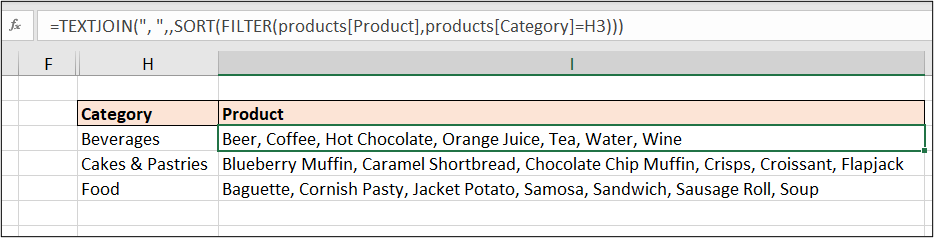
This formula uses the same FILTER formula as before.
The SORT function is wrapped around it to order the returned values. By default, the SORT function will order values in ascending order, so there is no need for additional arguments.
The TEXTJOIN function is then added to combine the results into a single cell. This is a terrific function that concatenates an array or range and separates them by a specified delimiter. In this example, a comma and space have been used. The second argument is omitted. This will ignore empty cells, which is not a factor in this scenario.
This formula does not spill, so the formula will need to be filled down to cells I4 and I5.
Lookup Multiple Values and Sort by Another Column
In this example, we have a table named ‘tblOptions’. In the table, we have some individuals and they are choosing the location they want to attend. They can choose a first, second and third option in order of their preference.
In column F, we have a sorted and distinct list of names taken from the table using the following formula.
=SORT(UNIQUE(tblOptions[Name]))
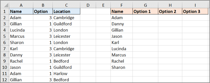
We want to lookup the three chosen locations for each individual and return them to the range beginning in cell G2. The returned values need to be in the order 1, 2, 3.
Let’s start with the FILTER function and use it just like the previous examples. This formula returns the three locations for the first name, which is Adam.
=FILTER(tblOptions[Location],tblOptions[Name]=F2)
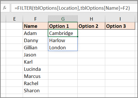
So, the FILTER function returns the locations, but we need to transpose the results to go along a row, and not down a column.
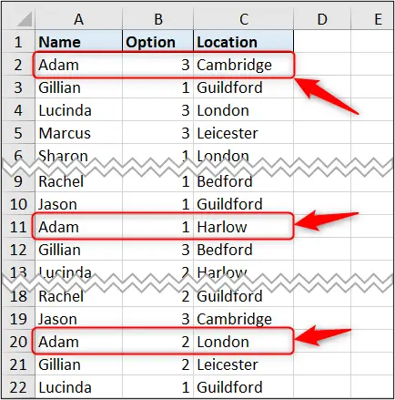
We also need to sort the results by the ‘Option’ column. For Adam, Harlow was his first choice, London was second and Cambridge was third.
The following formula achieves these objectives.
=TRANSPOSE(
SORTBY(FILTER(tblOptions[Location],tblOptions[Name]=F2),
FILTER(tblOptions[Option],tblOptions[Name]=F2))
)
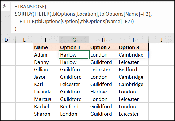
The SORTBY function is added to FILTER to sort the results by a column outside of the column used by FILTER. This is because FILTER is using the ‘Location’ column but we need to sort by the ‘Option’ column.
A second FILTER is used within the array to sort by argument of SORTBY. These are shown on different lines of the formula to help distinguish them. This second FILTER provides the three options for the specified individual.
The TRANSPOSE function is then added to return the results along a row.
So, this tutorial showed three examples of using a formula to lookup multiple values in Excel. We then explored how to combine the results into a single cell, or along a row, and also order the results.


Leave a Reply