In this blog post we create a reverse FIND formula to extract text after the last occurrence of a character.
Many of you reading this may already be familiar with the FIND function. You would probably have used it with LEFT or MID to locate a delimiter character, and return text before, or after that character.
In this tutorial we want to extract text after the last occurrence of a character, so want to create a reverse find effect.
Watch the Video – Reverse Find Formula
The Reverse FIND Excel Formula
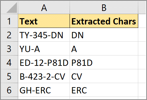
In this example, we are working with the data below in column A. We wanted to extract the text after the final hyphen character.
Each cell contains a varying number of hyphens, so we need to identify the position of the last occurrence of the character, and then extract the text.
The completed Excel formula for this reverse string search is shown below.
=RIGHT(A2,LEN(A2)-FIND("*",SUBSTITUTE(A2,"-","*",LEN(A2)-LEN(SUBSTITUTE(A2,"-","")))))
This formula is a monster so a detailed explanation is shown below. The video above also explains it step by step.
Find the Total Occurrences of the Character
The first job on our hands is to return the total occurrences of the hyphen character.
Our ultimate aim is to retrieve some text after the last occurrence, so we need to know how many there are in total.
The formula below uses the SUBSTITUTE function to replace all occurrences of a hyphen with nothing. A LEN function is used to count the number of characters remaining when the hyphens are removed.
This value is subtracted from the total number of characters in the cell, leaving us with the answer to the total number of hyphens.
LEN(A2)-LEN(SUBSTITUTE(A2,"-",""))
Replace the Last Character with a Unique Marker
We will now replace the last occurrence of the hyphen with a unique character, which we can then use to easily extract the text we want.
An asterisk (*) has been used in this example as the unique marker. It could have been any text character.
The brilliant SUBSTITUTE function is used to accomplish this, with a little help from some friends.
The previous part of the formula has been used in the instance number argument of the SUBSTITUTE function, to specify to replace the last hyphen.
SUBSTITUTE(A2,"-","*",LEN(A2)-LEN(SUBSTITUTE(A2,"-","")))
Extract the Text after the Final Delimiter Character
Now that we have inserted a unique marker in the position of the final delimiter character, it is time to find it and extract the text we want.
The following formula was added to what we have from the previous step. The ??? represents the formula part from the previous step.
=RIGHT(A2,LEN(A2)-FIND("*",???))
The RIGHT function is used to extract text from the end of cell A2.
To calculate the number of characters to extract, the LEN function returns the total characters in the cell. And then the FIND function locates our unique marker character.
The position of the marker character is subtracted from the total characters in the cell.
The final formula is as below.
=RIGHT(A2,LEN(A2)-FIND("*",SUBSTITUTE(A2,"-","*",LEN(A2)-LEN(SUBSTITUTE(A2,"-","")))))
This can be adjusted to return text from the second from last delimiter, or anything you want really.
You now have a way of searching a string from right-to-left, in addition to the typical left-to-right search.
Related Excel Formula Tutorials
- How to use the TEXT function of Excel – with examples
- Extract the postcode from a UK address
- 4 amazing tips for the CONCATENATE function
- 4 ways to separate text in Excel


My goodness it takes a devious mind to figure that one out. Congratulations! But it would have been so much easier if Microsoft had thought to write a FINDRIGHT function.
Thank you, John ?
Hi Alan
Thanks for the response. I am in Melbourne, Australia and I have responsibility for the Action Network member database for a group of environmental activists called “Lighter Footprints”. The data comes from a Google Groups list and about half the members do not have a last name entry, about 10% have only an email address. I am trying to clean up the data. This formula finds those with dots or spaces in the first name field and peels off the surname. As you can see it owes a lot to your “reverse find”:
=IF(AND(ISERROR(FIND(” “,A73)),ISERROR(FIND(“.”,A73))),””,IF(ISERROR(FIND(“.”,A73)),RIGHT(A73,LEN(A73)-FIND(“*”,SUBSTITUTE(A73,” “,”*”,LEN(A73)-LEN(SUBSTITUTE(A73,” “,””))))),RIGHT(A73,LEN(A73)-FIND(“*”,SUBSTITUTE(A73,”.”,”*”,LEN(A73)-LEN(SUBSTITUTE(A73,”.”,””)))))))
I was very delighted to find that someone had solved the exact problem that I was facing.
Cheers – John
Wow! That is one heck of a formula, John ?
Thank you! Worked perfectly for me to strip-off the data from the right side of a text string, collecting only those characters that proceed the final “space”. Just had to make one replacement in the formula, from “-” to ” “. Saved me much time on thousands of records. Bravo!
Great to hear, Adam. Happy to help.
Love this! It was exactly what I needed and further confirms my view that there is no problem that can’t be solved with an Excel formula 🙂
In my case I was looking to extract a number from a text string after the final space in that string. The text is imported from a PDF so has all sorts of nasties – using CLEAN(TRIM(A2)) in the formula place of A2 took care of any spurious leading or trailing spaces and so on.
Excellent, Robin. Glad it helped.
If you have Excel 365 you have to use “~” in the search function. So the proper form is FIND(“~*”…
Using VBA this is very simple
1. enter developer mode
2. add a new module
3. enter the following code:
Option Explicit
Public Function FindRev(r As Range, value As String) As Integer
FindRev = InStrRev(r.value, value)
End Function
Now you can use the FindRev function in your spreadsheet
Hi, thanks a lot!!!! This is brilliant! You are brilliant! I didn’t even know substitute can replace 1 instance! This reduces my work and thanks a for teaching me something new that would be useful in future as well 🙂
Blesssinngggss good wishes to you!!
You’re welcome. Glad I could help.
As for Excel 365 nowdays (Feb 2023) this task can be done with built-in excel function “TextAfter” like this:
=TEXTAFTER(A2;”-“;-1)
A2 = The string
“-” = Delimiter
-1 = Starting Postion . Use of minus signs means start from the end.
Absolutely. The new TEXTBEFORE and TEXTAFTER functions are awesome!
Try this
in A1: C:\Folder\another\12. specialname\And here the filename.txt
in B1: =IFNA((MATCH(“\”;MID(A1;SEQUENCE(LEN(A1);;LEN(A1);-1);1);0)-1);LEN(A1))
in C1
=MID(A1;LEN(A1)-(B1-1);999)
The IFNA is to prevent errors when no “\” is there.
String2Search BackwardsPosition\ Basename
C:\Folder\another\12. specialname\And here the filename.txt 25 And here the filename.txt
Fantastic work. Thanks.
Thank you, Josh.
Amazing trick, it is really!!
Thank you.
Some serious thinking went into that. Thanks for sharing!
My please. Thank you.