In this post, we look at a neat Excel VLOOKUP trick to select a column for the data to return instead of specifying a column index number.
This is one of the biggest frustrations for beginners to VLOOKUP and for users who work with wide data sets. Counting the columns to enter the correct index number is not ideal.
Well, this simple trick removes that hassle and will mean you only have to click the column now. Let’s see how to do this.
Watch the Video
Excel VLOOKUP Trick to Select the Return Range
In this example, we have a table of product sales and we want to return the category and the price of the product sold from another table.
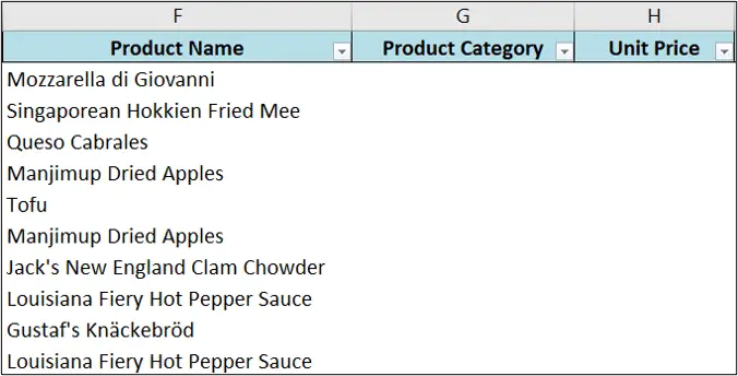
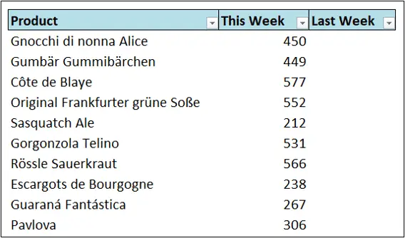
This is a snapshot of the product sales table with the empty columns ready for VLOOKUP to fetch the necessary information.
And this is the table named Products. The information we want can be seen in columns 2 (category) and 3 (price).
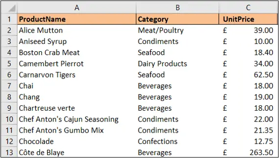
This is a small sample dataset. But the technique would be exactly the same even if we needed the data from column 60.
Download the completed Excel workbook to try it out for yourself.
To return the product category, the following VLOOKUP function would typically be used.
=VLOOKUP($F2,Products,2,FALSE)
This VLOOKUP searches for the product name (cell F2) in the Products table and returns the data from column 2.
This is easy when it is the second column, but let’s see the trick to make it just as easy with large tables.
The COLUMN Function
The following VLOOKUP formula uses the COLUMN function. The COLUMN function returns the column number from a given reference. The table column Category was provided by simply selecting it..
=VLOOKUP($F2,Products,COLUMN(Products[Category]),FALSE)
Although this example uses a table column, you can also select the sheet column B or a cell such as B1. The formula would work the same.
It is also important to be clear that although a table column is used, it still returns the column from the sheet, not the table.
So, if the table starts in column B. Then the second column of the table is column 3 of the sheet. And 3 is what the COLUMN function would return. This can be worked around by simply adding -1 after the COLUMN function.
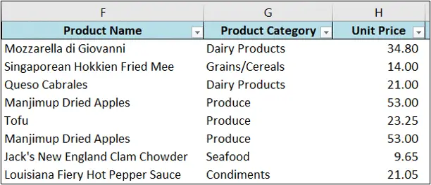
By adding this small and simple Excel function we were able to avoid the frustration of counting columns or using a more advanced technique to return it.
We can then copy the formula over to column H to return the product price also. The column will adjust relatively from column 2 to 3. Brilliant if the columns to return are adjacent like they are in this example.
Return the Last Column from a Table
Let’s look at a second example, but with a little difference.
In this example, we have the following table named Sales. It has products and then the weekly sales values across the columns.
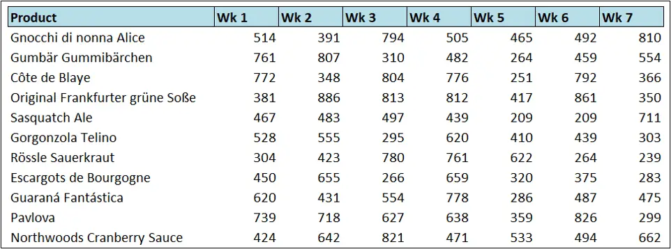
We have the following report table and we want to return the last week sales. So, this will be whatever the last column in the Sales table is. Currently it is week 7, but next week it will have changed to week 8.
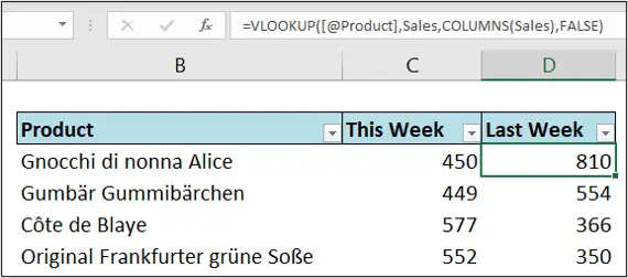
The following formula uses the COLUMNS function to return the number of columns (last column) from the Sales table.
=VLOOKUP([@Product],Sales,COLUMNS(Sales),FALSE)
VLOOKUP then uses this to return the value from the last column in the table.
Once again, table references are used because I’m a huge fan. However, the COLUMNS function will return the number of columns from any given range i.e. C:G or B3:G9 would also work.
To be clear, it is the number of columns from the range, and nothing to do with the sheet. So, in the range B:D there are 3 columns.


Leave a Reply