Excel does not display negative time. So if you are working with negative times, there is a problem. Fortunately, there are ways to work around this issue.
This tutorial will show two ways to display a negative time in Excel.
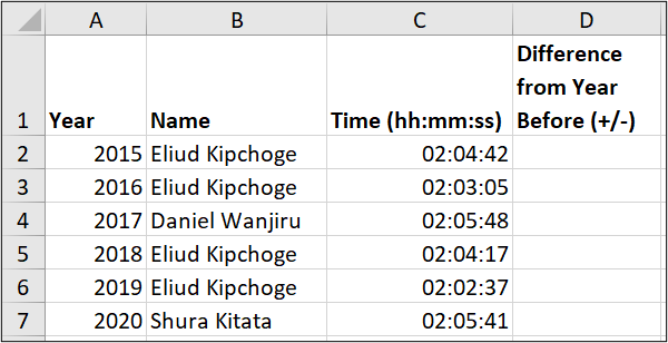
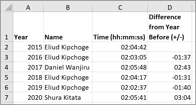
For this example, we have the fastest times for the last six London Marathons for the men’s category. And we want to see the time difference compared to the previous year.
If the time is faster than the previous year, the result will be a negative time. A slower time would return a positive time.
Download the Excel workbook to follow along.
Negative Time in Excel
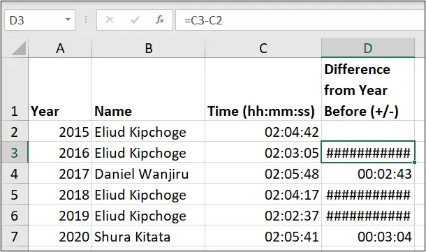
To calculate the time difference, the following formula has been used in range D3:D7.
=C3-C2
The negative times are shown as #######. This is not good enough, so let’s explore how to fix this.
Method 1: Using the 1904 Date System
One method is to change Excel from it’s 1900 system to the 1904 date system.
Doing this will enable Excel to display negative times correctly. However, this can have a negative effect on any dates you may have on the spreadsheet.
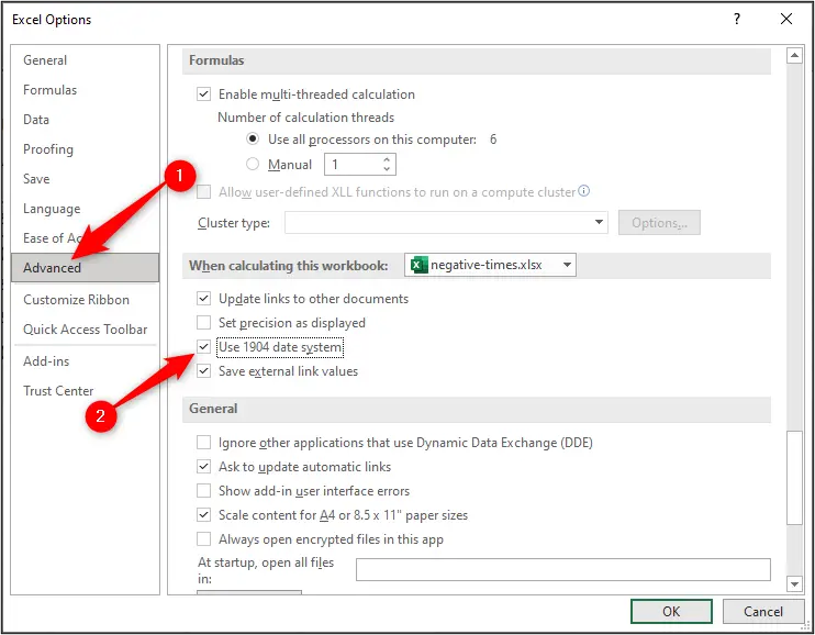
To change the date system;
- Click File > Options.
- Click the Advanced category.
- Scroll down the list of options and check the Use 1904 date system box.
This successfully corrects the negative times in column D.
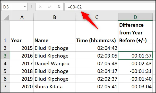
This is a super solution if you do not have other dates on the spreadsheet. If you do, these existing date values would be changed to four years in the future.
Method 2: Using the TEXT Function
An alternative method is to use a formula. To display the negative time in Excel with a minus sign “-“, we will use the TEXT function. This awesome function allows us to convert numbers to text but still apply number formatting.
The following formula uses the IF function to test if the result is a positive value. If so, the TEXT function is used to display the resulting time without the hours (the time difference would never be greater than 60 minutes).
If the result is negative, then the TEXT function is used along with the ABS function to display the negative time in Excel. The ABS function returns the absolute value, without regard for its sign.
=IF(C3-C2>=0,TEXT(C3-C2,"mm:ss"),TEXT(ABS(C3-C2),"-mm:ss"))
This method does produce a text result, so is limited if you want to perform further mathematical calculations on that column.
We could have used the ABS function alone to return the result as an absolute value. Then used Conditional Formatting to present the time in different colours to identify the positive and negative values. This would have maintained its numeric status.
One of the many things that make Excel so exciting is the different approaches to a challenge. In this example, I opted against the use of colour and really wanted a negative sign to to be shown.


What if I want to just input a negative time without comparing 2 different times?
without changing to 1904 so that it messes with actual dates in the entire spreadsheet and some complex formula.
Hi Bob, I’m not sure there is a way around this except – using the 1904 dates system as you say, and then dealing with any affected dates (only need to do this once). Or let Excel doing whatever time maths you are doing to require a negative time.
Unfortunately, as Excel does not recognise negative time, we are in a pickle, and they are the two options, I believe.
Try using Mod e.g. =MOD(C3-C2)
I’m not sure what this is referring to. MOD would need a second argument too for a divisor.
What if you want to do both display the – sign and use conditional formatting? I have tried everything I can think of to make the -HH:mm results turn red. I can get the + ones green just fine using the formula you gave, just not the negatives.