Display a Symbol Conditionally using the IF Function

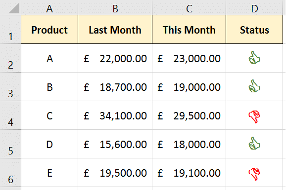
This blog post looks at using the IF function to display a symbol conditionally in a cell. In the image below a thumbs up or thumbs down symbol is shown dependent upon whether the sale of products have improved since last month.

This tutorial will show you how to display any symbol though, so you could insert a smiley face, hour glass, aeroplane and much more.

Find out the Letter or Number for your Symbol

The first thing we need to do is find out the letter or number for the symbol we want to insert. Every symbol from the Wingdings libraries has an associated letter or number when displayed in a normal written font such as Calibri or Arial.

To find this out; start by inserting the symbol in a cell on your worksheet. Then select that cell and change the font to Calibri, Arial or some other written font.

The letter or number will now be displayed instead. For example, the smiley face symbol is J, and the hourglass is 6. Importantly for this tutorial, we know the thumbs up symbol is C, and thumbs down is D.

Writing the IF Function to Display the Symbol

The following formula was written in cell D2 of the worksheet shown above.

=IF(C2>=B2,"C","D")

It tests if the value in C2 (this months sales) is greater than or equal to the value in B2 (last months sales). If it is then display C (remember this is the thumbs up symbol), and if not display D (thumbs down symbol).

Now that we have the IF function showing the correct value, all the cells containing the formula need to be formatted in a font such as Calibri to show the symbol.

Show the Symbols in Green and Red

In the example shown above, the thumbs up symbol is formatted in green, and the thumbs down symbol in red. This is done using Conditional Formatting.

1. Select the range of cells containing the symbols.
2. Click the Home tab and then Conditional Formatting.
3. Select Highlight Cells Rules and then Equal To.
4. Enter C in the first box and then select a green font colour from the Custom Format options in the second box. Click Ok.

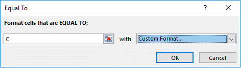
5. Repeat these steps to display in a red font if the value is equal to D.

Displaying a different symbol based on the values of your worksheet, and applying automatic custom colours can add a creative wow factor to your spreadsheets.

Depending on the kind of data you work with, there are loads of symbols on offer and they may just have your spreadsheets jumping out of the screen.

Watch the Video

More Related Tutorials

• Check if a Value is an Even Number
• Apply Conditional Formatting to Charts – Two Examples
• 5 Alternative Reasons to Use the COUNTIF Function
• Display the Sheet Name in a Cell using an Excel Formula