Create a five star rating system in Excel using Conditional Formatting. This can be a useful way of visualising ratings like you see on eBay and Amazon.
Watch the Video – Star Rating System in Excel
How it Will Be Done
The Conditional Formatting feature of Excel has a 3 star rating option. However, we would like a 5 star rating system. So, we will need to be clever and use another technique.
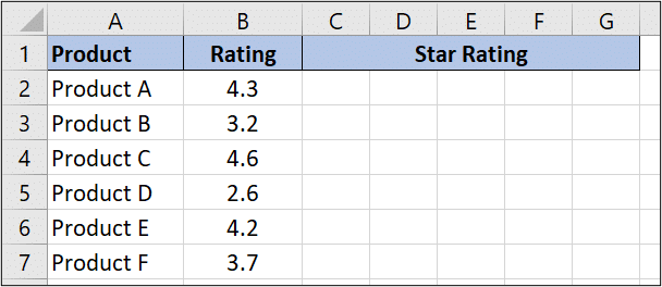
In the image below I have 6 products with an average rating for each. There are then 5 columns, one for each star.
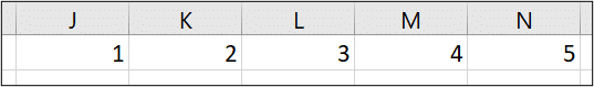
I have entered numbers 1 to 5 in cells J1:N1.The reasons for this will be clear when we start writing the formula.
We will write a formula in each cell to calculate that part of the average score. Then the Conditional Formatting tool will insert the stars.
Writing the Formula for the Star Rating System
The following formula was used in cell C2 and copied to the other cells of the table.
=IF($B2>=J$1,1,IF(INT($B2)=J$1-1,MOD($B2,1),0))
The end result is this.
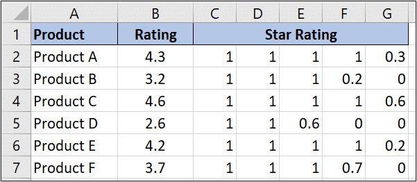
The first IF function tests if the rating is a greater number than the value in cell J1, and if it is, it puts a number 1 into the cell. As the formula is copied from cell C2 to D2 and E2 etc. The formula is tested against the values in cell K1, L1 etc.
The first rating has a number 1 in cells C2 to F2 because 4.3 is greater than the numbers 1, 2, 3 and 4.
The MOD function has been used to extract the decimal part of the rating. For the first rating this is 0.3. This is returned to the cell when the rating falls short.
Applying the Star Rating
To apply the Conditional Formatting rule,
- Select range C2:G7.
- Click Home > Conditional Formatting > New Rule.
- Select Icon Sets from the Format Style list, and then the star rating from the Icon Style list.
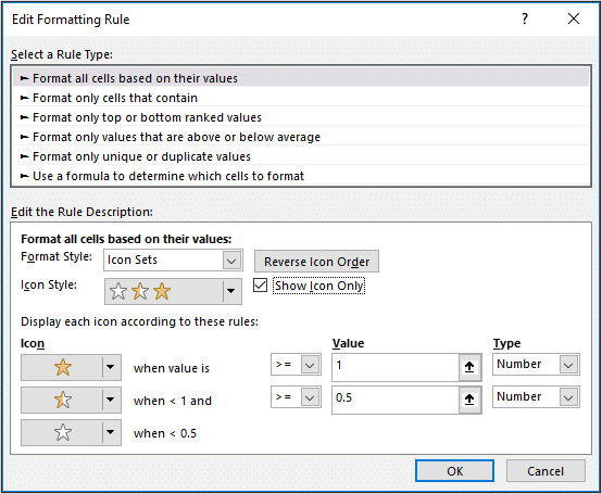
- Complete the Conditional Formatting rule like the image below. A full star is shown if the value is greater than or equal to 1, a half star if the value is greater than or equal to 0.5 and a blank star is less than 0.5.
- Select the Show Icon Only box to hide the formula results.
The completed five star rating system looks like this.
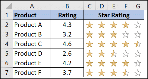
If you have to work with reviews and feedback this can be a neat way for visualising these responses.


How is the MOD function applied in this case?
The MOD function extracts the decimal part of the value. The value is divided by 1 and MOD returns the remainder.