Excel contains 500+ functions and this list is constantly growing. There are functions to perform almost any task including financial functions, date and time functions, and statistical calculations.
This post looks at 3 little known special Excel functions that will take your skills to another level and make you the envy of your work colleagues.
CHOOSE
The CHOOSE function in Excel returns a value or performs an action from a list of values based on a specified position. For example it may sum a range or lookup a different table based on user selection.
The syntax for the CHOOSE function is:
=CHOOSE(index_num, value1, [value2], …)
index_num – Specifies which value in the list of values that you want. It can be entered as a number between 1 and 254, a cell reference or a formula.
value – 1 to 254 values that the index_num will be selected from. They can be numbers, text, cell references, named ranges or formulas.
CHOOSE Function Example
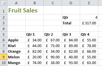
The example below shows the CHOOSE function (cell E3) being used to sum the fruit sales by quarter dependent on the user selection in cell E2.
=SUM(CHOOSE($E$2,B6:B10,C6:C10,D6:D10,E6:E10))
See more CHOOSE function examples in this video.
DGET
The second of these special Excel functions is the DGET function. The DGET function is a database function in Excel that will look up and retrieve data from a table.
It is very powerful and can retrieve data based on multiple conditions making it more effective than the likes of the more famous VLOOKUP function (in specific instances).
The DGET function is written as below.
=DGET(database, field, criteria)
Database – The range of cells where you want to search for and retrieve the data. The first row must contains the headings for each column.
Field – The column containing the information that you want to return. This can be entered as the column’s index number i.e. 5, or you can use the column heading enclosed with quotation marks e.g. “Salesperson”.
Criteria – The range of cells that contain the conditions for your search. The first row must contain the column heading.
DGET Function Example
The following formula returns the salesperson that took order 11248.
=DGET($A$1:$F$800,1,$H$2:$H$3)
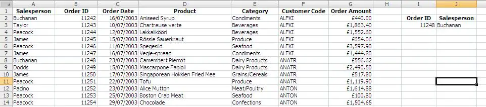
The formula looks within range A1:F800 and returns whatever data it finds in the first column. The criteria for the search is stored in range H2:H3. H2 contains the column heading of Order ID. This exactly matches the one found in row 1 of the database. Cell H3 contains the content to search for, in this case 11248.
Watch the Video
The OFFSET Function
The OFFSET function can be a confusing one to get your head around, but once you have it sussed it will take your Excel spreadsheets to new levels.
The OFFSET function returns a cell or range of cells that are a specified number of rows and columns from a starting reference.
Make sense? No? It didn’t to me either at first. Let’s break the function down and then see an example of its use.
Understanding the OFFSET Function
The formula is written as below;
=OFFSET(reference, rows, columns, height, width)
Reference: This is the starting point.
Rows: This is the number of rows you want to move from the starting point. Use a positive number to move down, or a negative number to move up.
Columns: This is the number of columns you want to move from the starting point. Use a positive number to move to the right, or a negative number to move to the left.
Height: The number of rows high that the range of cells you want to return is.
Width: The number of columns wide that the range of cells you want to return is.
The height and width arguments are optional. If they are not used then the width and height of the returned reference is the same as the starting reference.
OFFSET Function Example
Ok. Let’s see an example of the OFFSET function in action.
The most popular reason for using this function in Excel is to create a dynamic range. A range that will increase automatically as you add new rows or columns to your table of data. The video below shows it being used to create a dynamic SUM formula.
Using OFFSET to Create a Dynamic Range Name
Rather than nesting the function inside an existing formula such as SUM. Using the OFFSET function to create a dynamic range name is an awesome technique. Formulas and charts can then be based on this range name and will automatically update as the table of data changes.


Thanks!!