The OFFSET function in Excel returns a value from a cell, or range of cells that are a specified number of rows and columns from another cell.
This function can be really useful for creating dynamic references for your formulas and charts. Here you can see a great example of OFFSET being used for a rolling chart.
The syntax for the OFFSET function in Excel is:
=OFFSET(reference, rows, columns, [height], [width])
| Argument | Purpose |
|---|---|
| reference | The starting cell reference from which the offset will be applied |
| rows | The number of rows to offset from the reference. Enter a positive number for the number of rows below the reference, or a negative number for the number of rows above the reference |
| columns | The number of columns to offset from the reference. Enter a positive number for the number of columns to the right of the reference, or a negative number for the number of columns to the left of the reference |
| height | The height, in number of rows, of the returned range |
| width | The width, in number of columns, of the returned range |
Returning a Value from a Cell
Take the example data below.
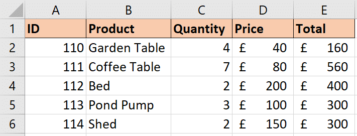
To return the value of £160 from cell E2, the following formula can be used.
=OFFSET(A1, 1, 4)
This will offset 1 row down and 4 columns across from cell A1.
Although the numbers are typed into the OFFSET function here. They could be returned by other functions, or form controls for more impressive examples.
Returning a Range using the OFFSET Function in Excel
In addition to returning a value from a cell, OFFSET can also return a range of cells. This can be really useful, because it can be used to feed other functions such as SUM.
=SUM(OFFSET(A1, 1, 4, 5, 1))
This returns the result of £1720.
It sums the Total column for all the products. The height and width arguments are used to select range E2:E6.
Returning the Last Value in a List
A very useful example of using the OFFSET function is to return the last value in a column, or a row. For this, we can insert the COUNTA function into OFFSET for more dynamism.
Take the example data below. This show a list of stock checks. And we want to return the value from the most recent check.
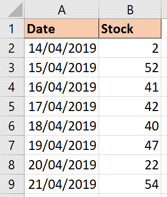
The following formula could be used.
=OFFSET(B1,COUNTA(B:B)-1,0)
The COUNTA function is used for the rows argument to find the bottom of the column. This moves 9 rows from B1 so a 1 is subtracted to make it the last cell in the column (instead of the first cell after the list).


