You may have multiple lookup tables for a VLOOKUP, and require the user to be able to select the desired lookup table.
The image below shows 3 lookup tables. The user is required to enter the product category to look for in cell B1, and then select the lookup table to use in cell B2.
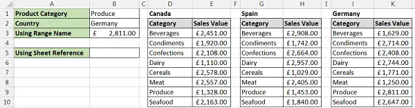
The VLOOKUP in cell B3 uses the content of cell B2 for its lookup table.
Creating this conditional lookup table will be achieved in 2 steps
- Define a range name for each lookup table. This name must match the exact wording of the selection in cell B2.
- Use the INDIRECT function in the VLOOKUP to convert the text from cell B2 to a reference to the defined name.
Defining the Range Names
In this example all 3 lookup tables are on the same worksheet. This is not necessary. Range names are unique for the entire workbook so the lookup tables can be on different worksheets if required.
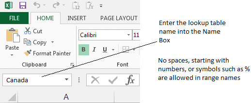
- Select the range of cells that make up the lookup table.
- Click in the Name Box, type the name you wish to use for the table and press Enter
Creating the VLOOKUP with Conditional Lookup Table
As mentioned the INDIRECT function will be used to reference the defined name dependent upon the selection made in cell B2.
The formula below creates the VLOOKUP with the conditional lookup table.
=VLOOKUP(B1,INDIRECT(B2),2,FALSE)
Using a Conditional Sheet Reference in the VLOOKUP Function
The following formula is an alternative to using defined names for the lookup tables. With each table on a different worksheet, the user selection in cell B2 can be used as a reference to the sheet the lookup table is on.
The INDIRECT function is used to convert the text in B2 to a reference to a worksheet.
=VLOOKUP(B1,INDIRECT(B2&"!A2:B9"),2,FALSE)
This formula used the concatenation operator (&) to join the text in cell B2 and a text string for the remainder of the table reference.


Leave a Reply