Excel ABS Function to Return the Absolute Value – and 2 Reasons Why

In this blog post, we will look at how to get the absolute value of a number using the Excel ABS function – and 2 examples WHY you might want to do that in Excel.

Lets start by defining what exactly an absolute value is.

An absolute value of a number is its distance from 0 regardless of its sign (positive or negative. For example, the absolute value is the same for 150 and -150 because the distance from 0 for both is 150.

Therefore, the most common reason in Excel to calculate an absolute value, is to convert a number from negative to positive within a formula.

The Excel ABS Function

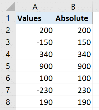
This is done using the ABS function. You can see a simple example of this function used below in column B to return the absolute value of each number in column A.

=ABS(A2)

Watch Two Useful Examples of the Excel ABS Function

Sum the Absolute Values in Excel

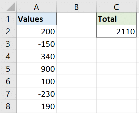
A real-world example could be that you want to sum a list of values.

And these values are a mixture of negative and positive. However you wish to sum the absolute values of those numbers, and not treat the negative values as negatives.

One way that we could do this, would be to embed the ABS function within a SUM function like below.

=SUM(ABS(A2:A8))

Because we are providing the ABS function with a range of cells, and not a single cell, this would need to be run as an array formula. So be sure to press Ctrl + Shift + Enter and not just Enter.

We could avoid an array formula though by using the SUMPRODUCT function instead. SUMPRODUCT is an array function and can therefore handle ranges of cells eliminating the need for Ctrl + Shift + Enter.

=SUMPRODUCT(ABS(A2:A8))

Check if a Number is Within a Tolerance Limit

Another useful reason to use the ABS function is to check if a number is within a specified tolerance level.

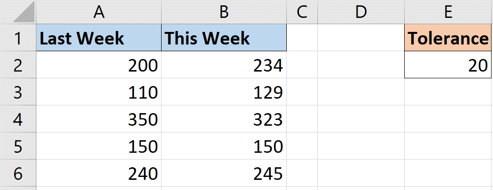
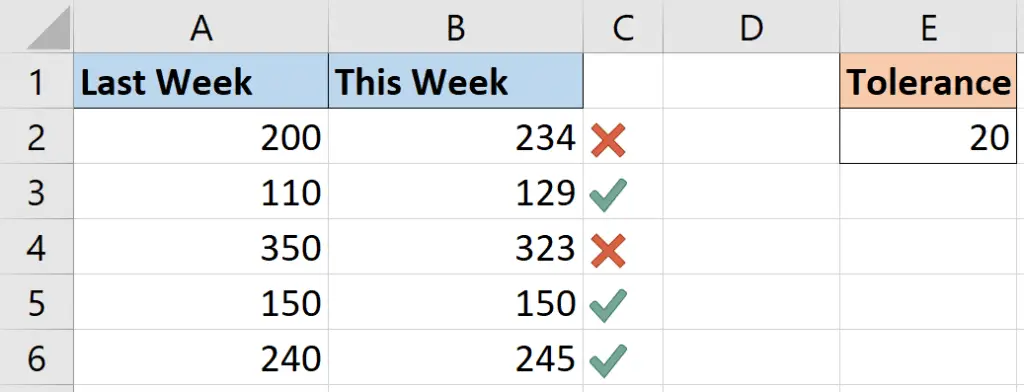
In the image below, we have some values from last week and some values for this week. And we need these new numbers to be within a range, or tolerance limit to last weeks. A tolerance of 20 has been set in cell E2.

In this example, the IF function will be used to test if the difference of the two numbers is within 20.

=IF(ABS(B2-A2)<=$E$2,"Yes","No")

The Excel ABS function is used because the difference of the 2 numbers might result in a negative value. But we need the absolute value to check if it is within tolerance.

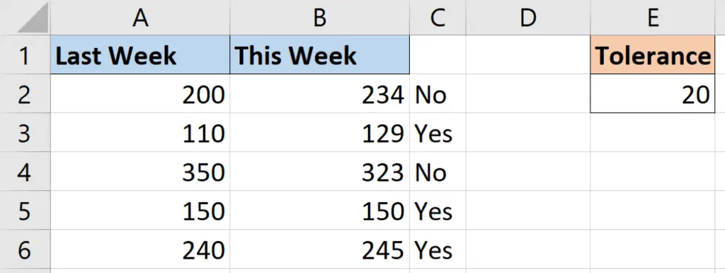
This easily identifies those within tolerance with a Yes, and those that are not with a No. The tolerance in cell E2 can easily be changed in the future if needed.

Adding a Conditional Formatting Rule

Maybe we wanted the result to be more visual by adding some Conditional Formatting. We can change the Yes and No to a 1 and 0 for easier testing.

=IF(ABS(B2-A2)<=$E$2,1,0)

I would like to add the green tick and red cross icon sets. So lets perform the following steps.

1. Select the range of cells (in this case its C2:C6)
2. Click Home > Conditional Formatting > New Rule (the following steps can be seen in the image below)
3. Select Icon Sets from the Format Style drop down
4. Select the green tick for the first icon, nothing for the second and a red cross for the third icon
5. Change the Type option from Percent to Number
6. Enter a 1 in the first box, and 0 in the second box
7. Change the logical operator to a greater than sign only in the second row
8. Check the box for Show Icon Only

The completed rule shows a green tick if the value is 1 or greater, and a red cross if 0 or less. It will also show the icon instead of the value.

This post showed two examples of why getting the absolute value could come in handy in the real-world. There are many.

However, it is typically when you need a positive number in a formula. Especially when subtracting value which might result in a negative that you do not want.