Shrinking Drop-Down List using Dynamic Array Formulas

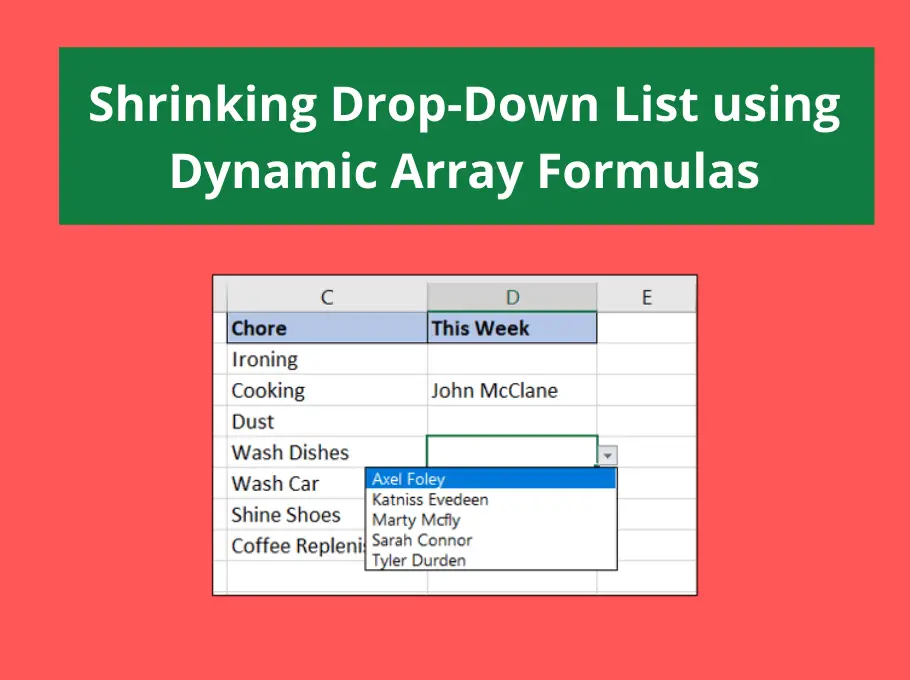
In this tutorial, we will create a shrinking drop-down list using the dynamic array formula engine and the FILTER function.

This is an awesome technique. Every time an item is chosen in the list, the list reduces and previously selected items are not shown.

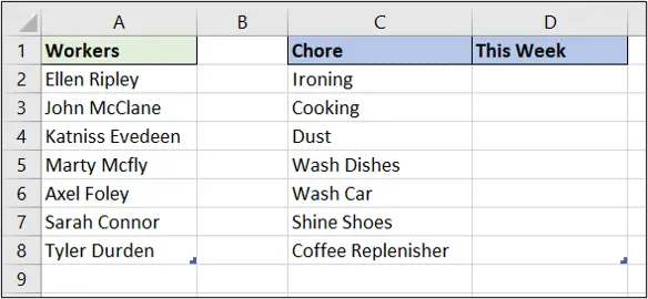
In this example, we have a table of workers and a table of chores.

We will create a drop-down list of workers names to assign to the chores. Each time a name is assigned the list will reduce to show only the remaining names.

Watch the Shrinking Drop-Down List Video

Formula to Determine if a Name has been Used

This first task is to write a formula that can determine when a name has been used in the chores table.

For this, I will use the fabulous COUNTIF function in column F.

The formula below counts the occurrences of the names in the chores table and returns a 1 for Axel Foley, the only name currently assigned to a chore.

=COUNTIF(chores[This Week],workers[Workers])

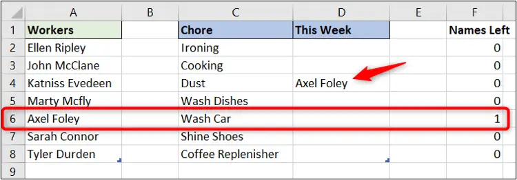
Enter the formula in cell F2 causes it to spill to the other cells in column F for the table height.

New to dynamic array formulas? Check out this video of 8 things you need to know.

Set the Logical Test

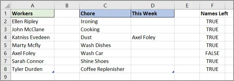
With the used names determined, we need to set the logic so that the names with a 0 should be shown in the list still.

So we will convert names with a 0 to display True with the following formula.

=COUNTIF(chores[This Week],workers[Workers])=0

Filter the List for Shrinking Drop-Down List Effect

Now we will add the FILTER function to the formula to filter the list to show only the unused names.

This formula filters the workers table by the criteria we have already set.

=FILTER(workers[Workers],COUNTIF(chores[This Week],workers[Workers])=0)

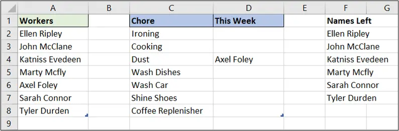
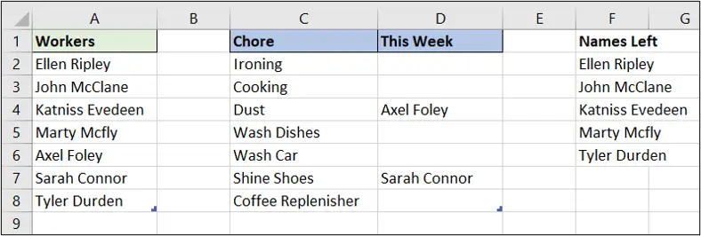
Every time a name is used in the chores table, it is removed from column F.

Sort the List

It may look like the list of names in column F is sorted, but it is just showing the names in the order that they appear in the workers table.

But what if the order of the names in the workers table was changed?

Let’s add the SORT function to the formula.

=SORT(FILTER(workers[Workers],COUNTIF(chores[This Week],workers[Workers])=0))

Now they will also appear in ascending order.

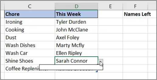
Create the Shrinking Drop-Down List

Now for the sexy part. Creating the shrinking drop-down list.

1. Select the ‘This Week’ column of the chores table.
2. Click Data > Data validation.
3. Select the allow a List and enter the following formula in the Source box provided.

=$F$2#

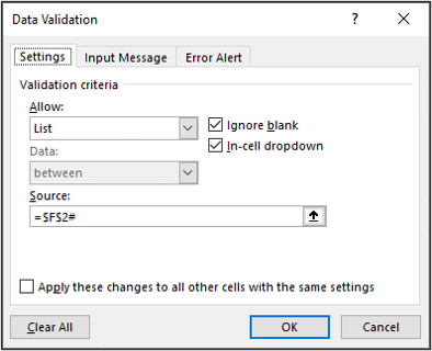
The # is the spill reference for dynamic arrays.

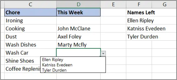
The list only shows the names available to work.

Hide Error Caused by no Names

If all of the names have been assigned to work, the drop-down shows the #CALC! error.

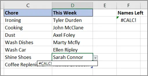
Now you shouldn’t really have to worry about this, because nobody should be using the list if there are no names left.

But maybe you are using this technique in a scenario where it does matter. Or you just want to tidy this up.

The IFERROR function can be added to show an empty string instead.

=IFERROR(SORT(FILTER(workers[Workers],COUNTIF(chores[This Week],workers[Workers])=0)),"")