This tutorial covers how to make table column references absolute. It will cover both table column and cell references.
Download the Excel workbook to follow along.
Table Column References Change
By default, table references are relative, so they change. This is a surprise to many users as a table reference looks absolute.
In the following example, the AVERAGE function has been used in cell F3 to average the scores for Maths. It looks like an absolute reference as it explicitly reads Grades table and the Maths column – Grades[Maths].

However, when this formula is filled to the right for English and Art. The formula changes.

In this example, this is good. We want this behaviour.
Make a Table Column References Absolute
Let’s look at an example where this behaviour is not desirable.
We have used the following XLOOKUP function in cell F2 to return the Name and Department for each ID from the table on the left, named staff. It does not work when copied into column G.
=XLOOKUP($E2,staff[ID],staff[Name])
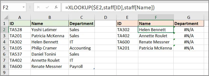
In this example, we need to make the staff[ID] column absolute, so that when it is copied into column G to the right, it does not change.
The staff[Name] column however, can be left relative, so that it moves to the Department column when the formula is copied.
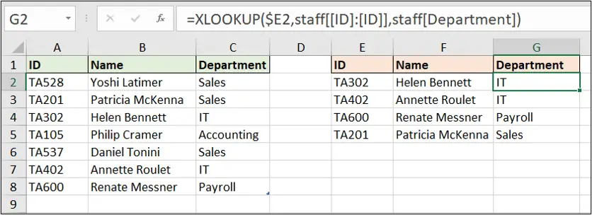
To do this, we change the staff[ID] reference to staff[[ID]:[ID]]. The complete XLOOKUP formula now looks like this.
=XLOOKUP($E2,staff[[ID]:[ID]],staff[Name])
So, the column header is repeated either side of the colon and an extra set of square brackets is added to enclose this range.
The following image shows the formula in column G with the table column reference unchanged.
Make a Table Cell Reference Absolute
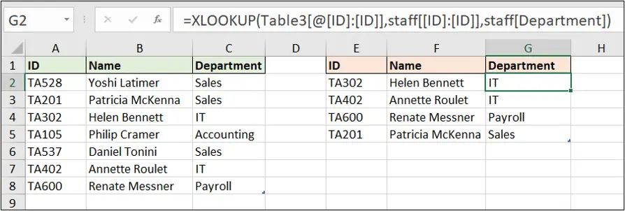
Now, let’s look at how we would make a single table cell reference absolute.
In this example, the table on the right that contains the XLOOKUP is formatted as a table. Because of this, the previous cell reference of $E2 has been changed to [@ID].
But we need to make this absolute, or it will move to [@Name] when we copy the formula to the right.
To do this, we follow the same approach as with the previous example, but ensure that the @ symbol is inside the first square bracket.
So, the [@ID] reference is changed to [@[ID]:[ID]].
=XLOOKUP([@[ID]:[ID]],staff[[ID]:[ID]],staff[Name])
Although we did not enter it into the formula, you can see the table name is added to the reference.
And nice and simple, that is how you can make a table column reference or a table cell reference absolute.


With respect to the staff exercise, you could also write in F2:
=INDEX(staff,SEQUENCE(ROWS(E2:E5)),{2,3})
All the cells in the F an G columns will be filled.
You said “However, when this formula is *filled to the right* for English and Art. The formula changes.”, but this didn’t work for me. When I copied the formula over, I used Ctrl+R. This does NOT update the structured table references to choose English and Art. It does work if you drag the handle of the cell with the formula in to the right. I’m a keyboard-heavy user so always used Ctrl+R to do this, rather than swap to the mouse and drag it.
Yes, this is true. Ctrl + R does prevent the relative behaviour. Thank you for mentioning this.
Excellent – answers exactly what I wanted.
And I love the Ctrl + R hint (pretty sure teh fill handle wasn’t around when I started Excel so have always preferred Ctrl R or D.
Awesome! Thanks, Robert.
This was an excellent tip. Thanks!
You’re very welcome. Thank you, Kristi.