Highlight the Cells that Contain a Specific Word (and it Matches Case)

In this blog post, we look at how to highlight the cells that contain a specific word. We will also ensure that the word in the cell matches the case of the word being looked for.

For this example, we have a list of the Ballon d’or winners of all time. Column B contains 3 letters in uppercase (after the name) which identify the country that the player represented at the time of winning the award.

In cell E1 I have entered the 3 digits for a country. I would like to automatically change the colour of all the cells that contain the country written in E1.

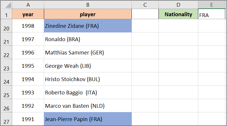
There is a good chance that the 3 digits identifying a country could also occur in a players name. For example, the letters for France – FRA do occur in the name Franz Beckenbauer.

To prevent this happening, we will match the case of the word we are searching for, as it is always written in upper case.

Watch the Video

You can watch the video tutorial of this lesson below.

Highlight the Cells that Contain a Specific Word

To achieve this we need to write a formula in a Conditional Formatting rule. The formula will identify if the country code occurs, then Conditional Formatting will highlight the cell.

Firstly we need to start a Conditional Formatting rule;

1. Select the Cells that you wish to format.
2. Click Home > Conditional Formatting and then New Rule.
3. Select the Write a formula to determine which cells to format option.
4. The formula below is then used in the box provided.

=ISNUMBER(FIND($E$1,B2))

5. Click the Format button and choose the formatting you want.

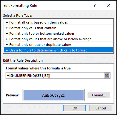
In this formula, the FIND function is used to search for the word in E1 in the cells of column B.

If a cell does contain the word, the FIND function returns a number specifying the position of the word in that cell. And if the word is not found #VALUE! is returned.

A number is not very helpful to us, so the ISNUMBER function is used to return TRUE if a number is returned and FALSE if not.

The Conditional Formatting rule will then run if TRUE.

Other Useful Tutorials

• Two Essential Conditional Formatting Tricks
• Applying Conditional Formatting to Excel Charts
• Techniques to Separate Text into Different Cells
• Count the Occurrences of a Character in a Cell