You may already be familiar with the Conditional Formatting tool in Excel. The amazing tool that automatically formats values tat meet specific criteria and improves how we visualise our data. Unfortunately, there is no Conditional Formatting with charts in Excel.
However, there is a way to create a Conditional Formatting with charts effect in Excel. And the great news. It is not that difficult. A simple IF function or other to perform a test and produce the required value for the chart is all we need.
This blog post will look at two examples of Conditional Formatting with charts so that you get a feel for how to do it. You can then apply the same technique to whatever example you need.
Highlight a Column Based on User Selection
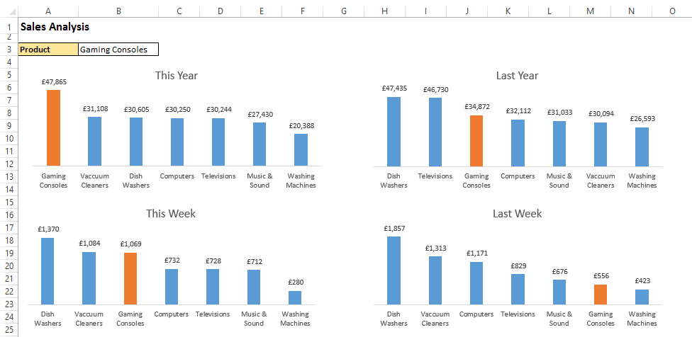
In the first example shown in the image below. We want to be able to highlight the column in each chart that corresponds to the product type selected by the user in cell B3.
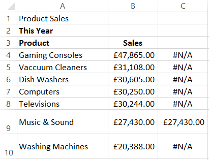
To achieve this we first need to add a column to the table which will show the value if the product type is selected by the user, but show the #N/A error if it is not.
The IF function is used to perform this logical test and required actions. The NA() function is used to return the #N/A error if it is not the product type selected. This is done because the chart will not plot error values, so it essentially hides those values on the chart.
The formula below is the one entered into cell C4. It compares the product name against the one selected by the user in B3 of the Sales By Product worksheet. It then displays the value in cell B4 if it is a match, or shows the error value if not.
=IF(A4='Sales By Product'!$B$3,B4,NA())
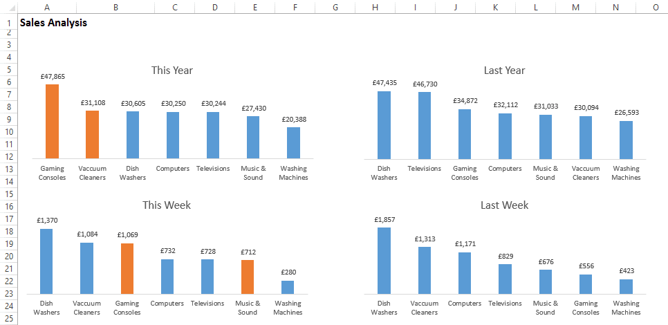
In this example, Music & Sound has been selected by the user.
This data range can then be selected to create a chart. In this example we create a column chart.
Select range A4:C10 and click Insert > Column Chart and select the 2-D Clustered Column. It should look like below.
The error values are hidden and only the column for the selected product type is displayed.
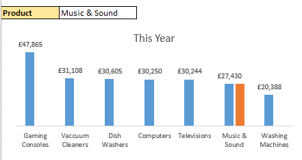
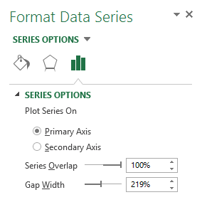
Double click on the conditionally highlighted column (the orange Music & Sound) and edit the Series Overlap to say 100%.
And our work is done. Continue to apply any further formatting that you think improves the chart.
Highlight the Columns that Show Sales Increase
In this example, we look at highlighting only the columns where the value represents and increase from last year, or last weeks data.
As you saw in the previous example, it is all about the IF function. We use a logical function like IF to perform the conditional test and only show the value if relevant.
Once we have this, we repeat the same chart technique as before to overlap the data series.
The formula below has been entered into cell C4. It compares the sale of this year (B4) against last years sales of the same product. Because the lists are in order largest to smallest by sales value, a VLOOKUP function is used to return the correct sales value.
=IF(B4>=VLOOKUP(A4,$E$4:$F$10,2,FALSE),B4,NA())
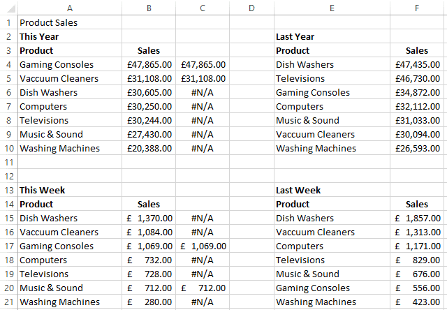
The end result looks like below showing only two products have increased sales since last year, or last week.
With this amazing technique you can apply any Conditional Formatting to charts in Excel. All the power comes from the logical function in the table.
Other typical examples might include highlighting actuals against target values, or the max and min values of a chart.
Watch the Video – Conditional Formatting with Charts
More Chart Tutorials
Two Essential Conditional Formatting Tricks You Need to Know
Create a Rolling Chart for the Last 6 Months
Create a Scrollable Chart for your Excel Dashboards


Leave a Reply