Interactive Checklist in Excel

In this blog post, we look at creating an interactive checklist in Excel. The checklist will automatically mark the items in a list when they are checked.

To do this we will first need to insert checkboxes onto the spreadsheet, we then need to be able to highlight an item when it is completed.

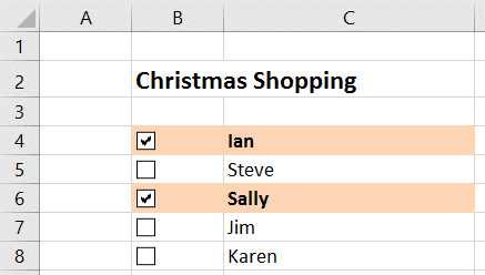
In this tutorial, I am using the idea of a Christmas shopping list of names (shown below). Your checklist could however be for any list of tasks, inventory or products.

Insert Checkboxes in Excel

To insert checkboxes in Excel, you need the Developer tab on the Ribbon. If you do not have this, right mouse click on the Ribbon, select Customize the Ribbon and then check the Developer box.

On the Developer tab, click the Insert button of the Controls group and then click the Check Box (Form Control) button.

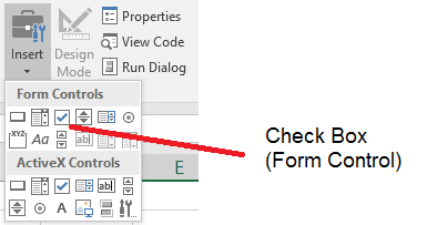
Click and drag to draw the checkbox onto the spreadsheet. Resize and position the checkbox so that is neatly fits inside a single cell. Right mouse click the checkbox and select Edit Text to change the default label. In this tutorial I have deleted the text next to the checkbox.

Select the cell containing the checkbox (not the checkbox itself) and copy and paste that cell to all the others in the list where you will need a checkbox.

You then need to link the checkbox value to a cell. Select the checkbox by pressing Ctrl and clicking on it. Then type = in the Formula Bar and select the cell you want to link the checkbox value to.

In this example, I have used cell A4. The font of column A has been set as white so the values are not visible to the user.

When linking to a cell only absolute cell references can be used such as =$A$4. Unfortunately this means you need to repeat this process for every checkbox in the list.

Watch this video to see how to create a macro that links all the checkboxes of a sheet to a cell saving lots of time.

When a box is checked this linked cell displays TRUE, and if not will display FALSE (or blank if unused). So column A will be used to know if a box is checked or not.

Automatically Format the Checked Items

With the checkboxes in place we want to automatically format the items when they are checked by writing a Conditional Formatting rule.

We will need a basic formula for this because the Conditional Formatting rule will refer to a cell outside the selected range.

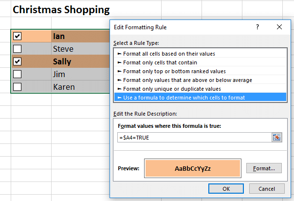
1. Select the range of cells that you want to apply the formatting to. In this example I selected the entire table, range B4:C8 in the image above.
2. Click the Home tab, Conditional Formatting and New Rule.
3. Select Use a formula to determine which cells to format, and enter =$A4=TRUE. In this example, cell A4 is the first cell in the table that contains the response from a checkbox click.
4. Click the Format button and choose what formatting you want to apply.

With the data in column A tracking the items to checked, you could take the interactive checklist in Excel further and create totals for how many items checked, or how many unchecked. You could even then show this information graphically. I have decided not to cover these extras in this tutorial though.

Watch the Video – Interactive Checklist in Excel