The VLOOKUP function will look down the leftmost column of a table and return a value from a specified column index number. To create a two way lookup formula, we will need something more flexible.
The INDEX and MATCH functions can be used to create a two way lookup that looks down a column and across a row.
These two functions used together create a very versatile and dynamic lookup formula. A far cry from the rigid structure of VLOOKUP.
If you are using Excel 365 or Excel 2021 version of Excel, you can also create a two way lookup with the XLOOKUP function. This is awesome and you should definitely check it out. But for now we will stick with the INDEX MATCH combination, and INDEX is the greatest function of all.
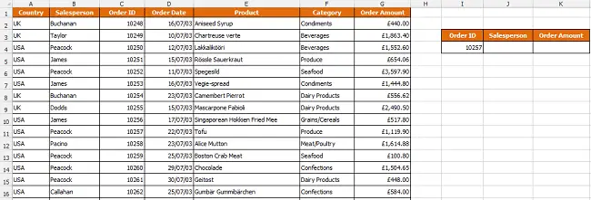
In the example, below we wish to look for an order using the ID, and return the salesperson’s name and the order amount using the same lookup formula in both cells.

The INDEX and MATCH Functions
The two way lookup formula is a combination of the INDEX and MATCH functions. These two functions are fantastic and have many uses in Excel. Let’s have a little look at the two of them first.
The INDEX function is used to return a value from a specified column and row. In addition to its use in a two way lookup, this function is used when working with form controls on a spreadsheet.
When used to return a value it is written as below.
=INDEX(array, row_num, [column_num])
This function wants to know the row and column number of the cell containing the value to return.
The MATCH function is the driving force in this formula. It will be used to find and return the row and column numbers for the INDEX function. INDEX can then return the value from that cell.
The MATCH function is heavily used in many lookup and reference situations to add extra muscle to the likes of VLOOKUP, or Conditional Formatting.
It’s structure is as below.
=MATCH(lookup_value, lookup_array, [match_type])
The lookup value is the value to search for.
The lookup array is the range of cells to search in.
Match type is the type of lookup to use. You can select an exact match, or one that finds the closest match if it cannot find the value you are looking for.
Create the Two Way Lookup Formula in Excel
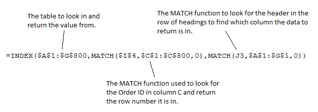
In this example, the formula below is entered into cell J4 and copied into K4.


Leave a Reply