Create a Case Sensitive Lookup Formula in Excel

Excel lookup functions such as VLOOKUP and MATCH are not case sensitive. They will not worry about matching the case of the lookup value and the cell entries when they search.

But what if you need the cases to match? Well let’s have a look.

Ensuring an Exact Match in the Lookup

To ensure we have an exact match we can use the EXACT function. This function compares two strings of text to see if they are the same, and if they are it returns TRUE, but if they are different it will return FALSE.

The EXACT function looks like this;

=EXACT(text1, text2)

Text1 and Text2 represent the two text strings that you want to compare. In our example these will be the lookup value, and the range of cells we are looking in.

Because we are going to be asking the EXACT function to test one piece of text against a range of text entries, our lookup formula will be entered as an array formula. This special type of formula is entered by pressing Ctrl + Shift + Enter, instead of just Enter and are sometimes referred to as CSE formulas.

Create a Lookup Function with Exact Match

The INDEX and MATCH functions will be used for the lookup in this example. These two functions offer a very versatile Excel lookup formula. If you use functions like VLOOKUP on your spreadsheets and are not familiar with these, I suggest checking them out. You will not be disappointed (Learn more about INDEX and MATCH)

In the example below, we want to return the city that a customer is based in from a list using the customer ID. We want to force the customer ID to be entered using the correct case.

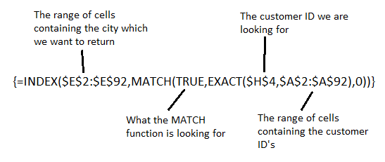
The Excel lookup formula below is used to create a case sensitive lookup for an ID entered in cell H4.

You do not type the curly braces when writing the formula. Excel will input these when you press Ctrl + Shift+Enter.

The MATCH function is looking for the value of TRUE. This is because the EXACT function has been used to test the customer ID against all the ID’s in column A. The value TRUE is returned if an exact match is found.

Watch the Video – Case Sensitive Lookup Formula