Conditional Formatting Multiple Columns – 3 Examples

In this blog post, we will explore using Conditional Formatting with multiple columns. And we will run through three different examples of doing so.

Conditional Formatting is typically applied to one cell, or column. It evaluates the cells in that range, and also applies the formatting to that same range.

In this blog post though we take things further to see example of testing and formatting multiple columns.

Using the AND Function with Conditional Formatting

In this first example we want to apply a Conditional Formatting to the data set below.

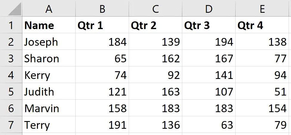
We want to format the row if every value in columns B, C, D and E is greater than or equal to 100.

1. Select the range of cells you want to format (B2:E7 in this scenario).
2. Click Home > Conditional Formatting > New Rule.
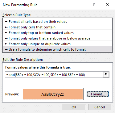
3. Select the Use a formula to determine which cells to format option.
4. Enter the formula below into the box provided.

=AND($B2>=100,$C2>=100,$D2>=100,$E2>=100)

The column are made absolute in the formula so that it does not move to each cell when we copy it to the right.

Click the Format button and choose what formatting you would like.

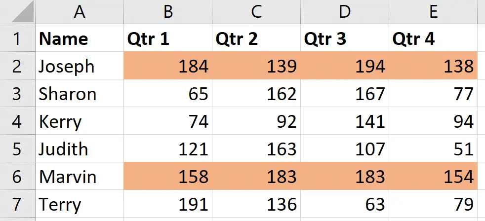
The finished article looks like below. Two of the persons met this target.

Testing a Threshold Value in a Another Cell

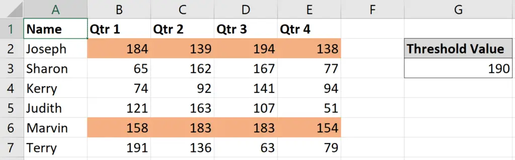
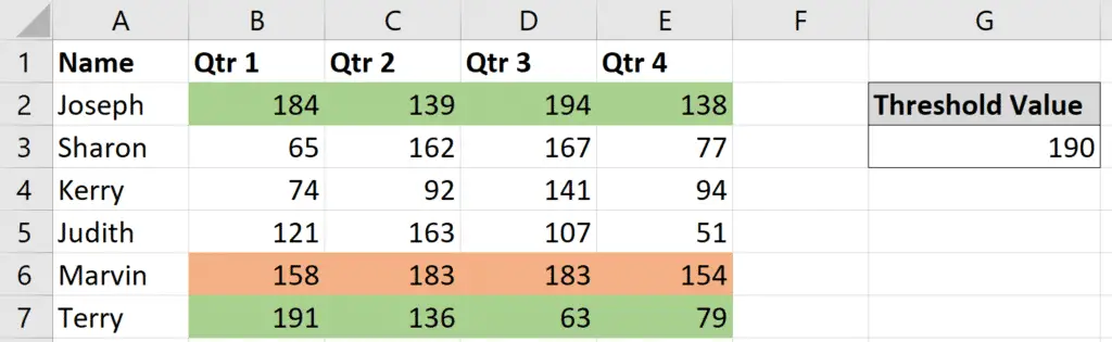
In this example, we would like to format the row if any one of the cells has a value greater than or equal to the value in another cell.

In the data below, we have a threshold value in cell G3 which we would like to test against. The Conditional Formatting rule from the previous example is also still applied.

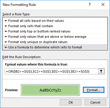
Because we are hoping to apply the formatting if any one of the cells is true – we will use the OR function.

Follow the steps from the previous example to create a new rule and enable us to enter a formula.

We will use the following formula. The reference to cell G3 is absolute.

=OR($B2>=$G$3,$C2>=$G$3,$D2>=$G$3,$E2>=$G$3)

The rule is applied to the dataset.

You can see that an additional row has been formatted, but it has also overwritten one of the rows from the previous example (Joseph).

Now, the previous rule was more important than this one. So we need to change the order of the rules so that if they are both true, then the rule with the AND function has priority.

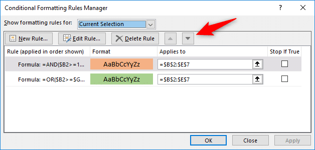
Click on one of the values in the range and click Home > Conditional Formatting > Manage Rules.

Use the arrows as indicated in the image below to change the order of the rules so that the AND function is on top. The higher in the list, the greater the priority.

Now this is what we wanted.

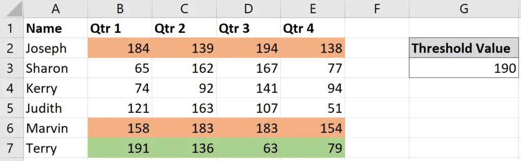
And if the value in cell G3 is changed. the Conditional Formatting rule will react to this.

More Than Two Columns Meet Criteria

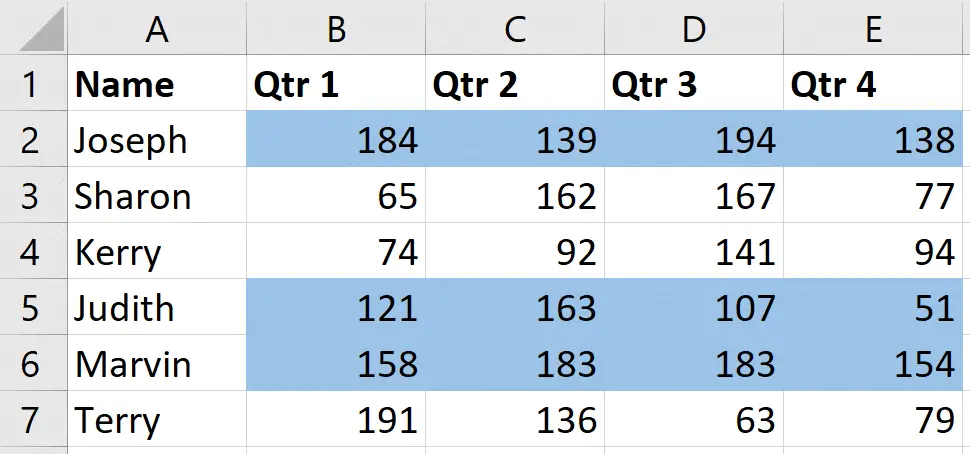
In this final example, we would like to apply the Conditional Formatting rule if more than 2 of the columns have values of 100 or more.

We will use the COUNTIF function for this.

This function can count how many cells contain a value of 100 or more. And then we can test if the answer to that is more than two.

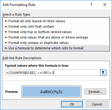
Follow the steps from the previous examples to create a new Conditional Formatting multiple columns rule using a formula.

The formula below can be used.

=COUNTIF($B2:$E2,">=100")>2

The rule is applied to the data range. The previous rules have been removed.

In this blog post we looked at three different examples of how and why to test multiple columns with Conditional Formatting.

I hope it has given you some ideas where you might be able to apply similar techniques.