Compare Lists with VLOOKUP

A common requirement in Excel is the need to compare two lists. In this tutorial, we will compare lists with VLOOKUP.

You might need to compare two lists to highlight missing records, highlight matching records or to return a value.

The VLOOKUP function can be used to compare lists in Excel by looking for a value from one list in another. You can then take the required action.

This tutorial shows how to compare lists with VLOOKUP. The VLOOKUP function can be used with other formulas, or Excel features, to accomplish different results involved with comparing two lists.

Combine with the IF Function to Return a Value

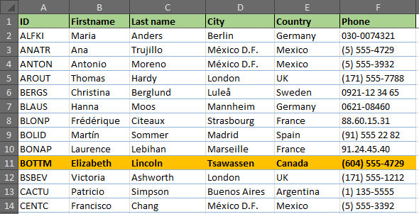
Let’s say we have two customer lists like the image below. Both lists are identical with the exception that list 1 has fewer customers than list 2.

We want to compare the two lists and identify the differences. The ID field will be used to check both lists as it is a unique field.

In this first example, we will look for the customers from list 1 in list 2 and return the text “Not found” if they are missing. If they are found in list 2 we will keep the cell blank.

The formula below uses the VLOOKUP function along with the IF and ISNA functions to achieve this objective.

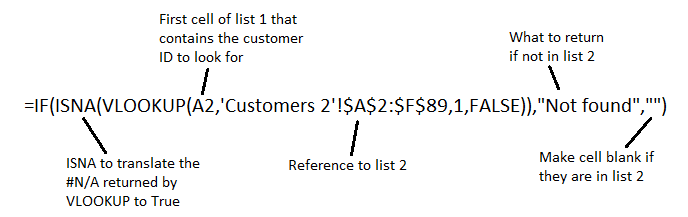
Let’s have a look at the role each function is playing in this formula.

VLOOKUP: The VLOOKUP function has been used to look for the customer in the second list and return the customer ID (specified as 1 in the formula).

If the VLOOKUP function cannot find the customer it returns the #N/A error message. This is what we are interested in as it means the customer is on list 1, but not on list 2.

ISNA: The ISNA function is used to detect the #N/A message brought back by VLOOKUP and translate it to True. If an ID is returned it returns False.

IF: The IF function will display the text “Not found” if ISNA returns True and will keep the cell blank if ISNA returns False. This function is used to take whatever action you want based on the findings from VLOOKUP.

Compare Lists with VLOOKUP to Highlight Missing Records

This formula can also be used with Conditional Formatting to highlight the differences between the two lists, instead of returning a value.

This example shows how to change the cell colour of the whole row of the table when a customer is missing from the second list. Formatting the entire row rather than just a single cell will make it clearer to identify the missing records, especially in a table with many columns.

1. Select all the cells of the table except the header row.
2. Click Conditional Formatting on the Home tab of the Ribbon and select New Rule.
3. Select Use a Formula to determine which cells to format from the top half of the window. In the bottom half enter the formula below into the box provided.

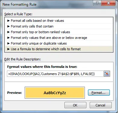
4. Click the Format button and choose the formatting you want to apply to the row of the missing records

Compare Two Lists and Highlight Matching Records

To compare the two lists and highlight the matching records, the NOT function will need to be added to the previous formula.

=NOT(ISNA(VLOOKUP($A2,'Customers 2'!$A$2:$F$89,1,FALSE)))

The NOT function is used to reverse the result of the VLOOKUP. So instead of highlighting the missing records it highlights the matches.

Watch the Video

There are many ways to compare lists in Excel. Formulas are great! Quick, versatile and keeping it on the grid. Merge Queries in Power Query is a fantastic alternative especially if the lists are coming from an external source.