Compare Two Lists in Excel to Highlight Matched Items

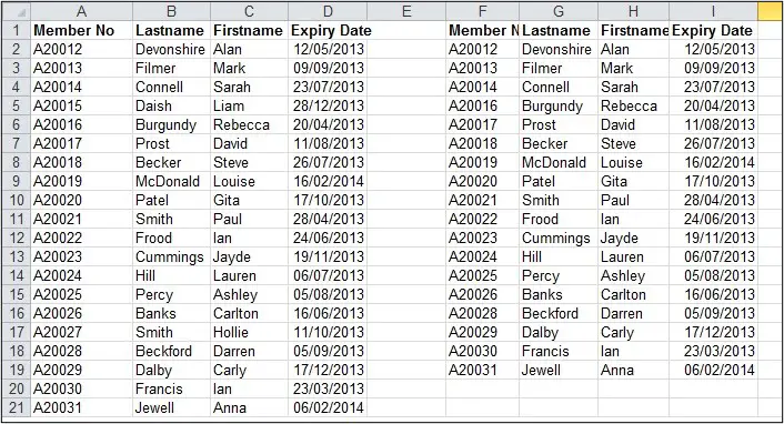
In this post, we will look at how you can compare two lists in Excel to highlight matched or unmatched items.

We will first identify the items that appear in both lists, and then look at how to highlight the items that appear in the first list but are missing from the second list.

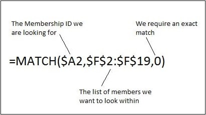
The MATCH function will be used to compare both lists and will return if a record is found, or is missing. The MATCH function returns the relative position of an item in a list. If it cannot find the item, it will return the #N/A error message (learn more about the MATCH function).

Compare Two Lists in Excel to Highlight Matched Items

1. Select the range of cells in the list you want to format.
2. Click the Conditional Formatting button on the Home tab of the Ribbon and select New Rule from the list.
3. Click the Use a formula to determine which cells to format option and enter the formula below in the box provided.

Because we are applying the Conditional Formatting to the entire row, the dollar signs are important to fix different elements of the cell references.

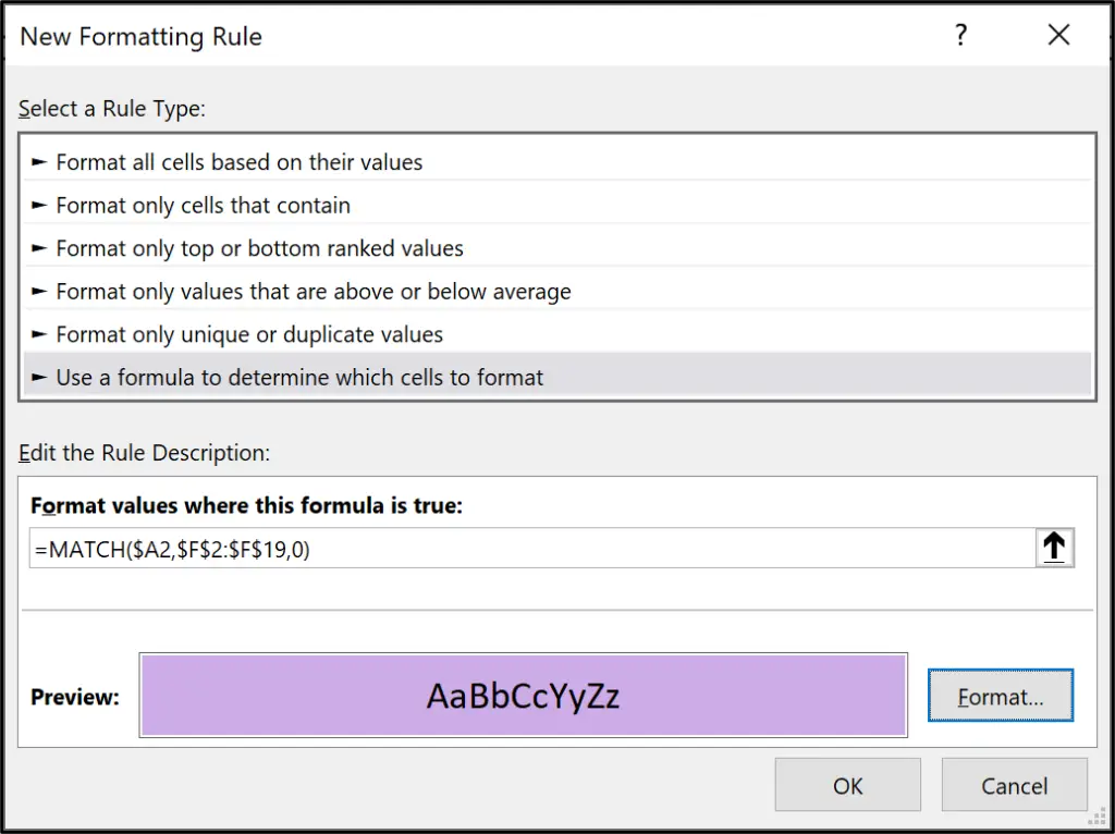
4. Click the Format button and select the formatting of your choice.
5. Click Ok

Compare and Highlight the Missing Items

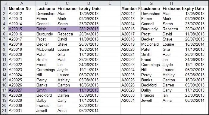
Instead of highlighting the duplicate items when we compare two lists, this function can be altered slightly to highlight the items that are unique to the first list.

Follow the steps as before but use the formula below for the Conditional Formatting rule.

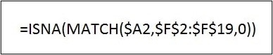
The ISNA function is used to return true if the #N/A error message is returned. Because #N/A is returned if the Match function cannot find a record, this formula identifies the missing items in a list.

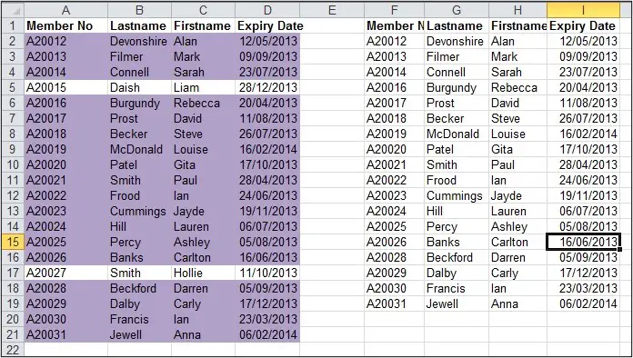
This tutorial showed how the MATCH function could be used to compare two lists and highlight matched or matching items.

Depending on the end goal, Excel offers a few methods to compare lists. Using Merge Queries in Power Query is a great alternative. The FILTER function with COUNTIFS is another.